Support Vector Machines and Neural Networks for Image processing - Part 2
This post forms the second part of the introductory material we covered during our sessions on SVMs and Neural Networks. Both posts are slightly more biased towards a probabilistic angle to build intuition.
Neural Networks
What are they?
Neural networks are models which behave as universal function approximators. This means that they can be used to model basically any function out there. Here we will look at an example of using them for a simple 2 class classification problem.
The neural network model is composed of basic units called layers. Each layer recieves a vector as input and produces a vector output. Let the input of a layer be \(x\), and its output \(y\). The simplest kind of layer is a dense layer. It just implements an affine transformation.
\[\begin{equation} y = W x + b \end{equation}\]Note that the above equation is a matrix equation, and \(W\) is called the weight matrix. The constant vector \(b\) added is called the bias vector. Note that the weights and biases of each layer are the parameters of the model. The goal is to choose these parameters such that the overall model best fits the data we have observed.
The simplest model is composed of 1 layer. The input and output to the model are \(x\) and \(y\) in the above equation. If \(x\) has a size of \(N\), and \(y\) has a size of \(M\), then \(W\) would be a \(M \times N\) matrix.
To make models with more parameters, we can cascade dense layers one after another. A model with two layers would look something like
\[\begin{equation} y = W_2 (W_1 x + b_1) + b_2 \end{equation}\]Note that the number of rows of \(W_1\) and \(b_1\) can be chosen by us arbitrarily, because the only constraints are on the rows of \(W_2\) and columns of \(W_1\), corresponding to \(M\) and \(N\). We can add as many layers as we want which are as large or small as we want.
Do you notice anything weird in the above discussion?
No matter how many dense layers you cascade, we can always simplify the model into one dense layer. So in essence, we aren’t adding any new capability to the model, as its output will always be linear with the input. To fix this issue, we have introduced some form of non-linearity in the model. This is done by applying a non-linear function to the outputs of each of the layers. Let us call this function \(\sigma (z)\). This function is called an activation function. Some commonly used activation functions are:
- The sigmoid activation: \(\sigma (z) = \frac{1}{1+e^{-z}}\)
- The hyperbolic tangent: \(\sigma (z) = \tanh (z)\)
- The rectified linear activation (ReLU): \(\sigma (z) = max(0,z)\)
Our new 2-layer model will now look like this:
\[\begin{equation} y = \sigma(W_2 \sigma(W_1 x + b_1) + b_2) \end{equation}\]Now, we have the ability to tweak the numerous parameters in the weight matrices and bias vectors to make the function from \(x\) to \(y\) look like almost anything we want. The more number of parameters we have to tweak, in general, will give us more control over how the total function looks. But too many parameters will not only make the computation slower, but can also cause overfitting, a problem which we will deal with later. The parameters of the neural network like the number of layers, how large the output of each individual layer is, and which activation function to use for each layer are called hyperparameters.
But why are these types of models called neural networks anyway? Well, we can interpret the model with a finer resolution. The values of vectors can be thought of as the outputs of small computational units called neurons. The neurons in the output of a dense layer can be thought of as units which multiply each of the incoming inputs by a corresponding weight and then add them all up along with a bias. Then, an activation is applied to this sum. The neuron then sends this value as its output. We can then represent our 2 layer model with the figure below:
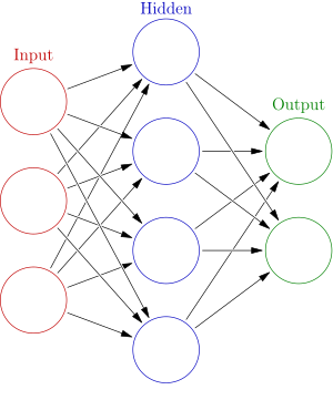
You can think of the two sets of arrows as the two weight matrices \(W_1\) and \(W_2\). This interpretation of the model draws analogies with how the brain works. The brain is supposedly an interconnected network of neurons whose electrical activations depend on the excitations given to them through the connections with other neurons. However, that’s as far as this analogy gets.
‘Training’ a neural network
Ok, so now that we have a model which can more or less approximate any function we want, how do we set the weights of our model to fit the function which we want ( this job is called training the model ). First, we need a measure of how good of a fit a particular set of weights will result in. We can evaluate this measure by giving our model some inputs and comparing the outputs of the model to the actual outputs we want. The set of inputs and outputs which we already have is called the dataset. So, the dataset can be represented as \((x_i,y_i)\). Suppose our model gives the output \(y'_ i\) when given an input \(x_i\). Ideally, \(y'_i = y_ i\) for all \(i\). But this will never be the case. So we have to look at how \(y_i\) and \(y'_ i\) differ. We can define a loss function on \(y_i\) and \(y'_ i\) which outputs one number representing how far away the two vectors are from each other. Our goal would then be to minimize the sum of this loss function over all the points in our dataset by varying the weights and biases of the network. Our job of training the network is now reduced to an optimization problem.
We solve this problem using the following approach. We find the output of the network to all the inputs from the dataset and evaluate the total loss using the outputs. We then find the gradient of the loss function with respect to ALL the parameters in the network. Then, we tweak the parameters to move in the opposite direction of the gradient so as to reduce the loss. We then repeat this process many times over all our samples until we reach a minimum in the loss.
There are a whole list of tasks in the above paragraph. They are as follows:
-
What loss function to use?
-
How to find the gradient of the loss with respect to so many parameters?
-
Suppose we could do the above, how much along the gradient should we move, and how are we sure that we will reach a global minimum?
-
Finding the outputs and gradients each time for all the data points would be extremely slow, is there anything better we can do?
Here are some short answers without detail, as these problems are not trivial.
-
The type of loss function we choose depends on what type of function we are trying to approximate.
-
Finding the gradient with respect to all these parameters is done using an ingenious algorithm called backpropagation. It is basically a repeated application of the chain rule.
-
We can’t always be sure that we will reach a global minimum. But it turns out in practice that a local minimum is pretty good too. Also how much to move along the gradient in each step is another hyperparameter called the learning rate.
-
To reduce computation we ‘batch’ the data. For each parameter update we will now only use a part ( a batch ) of the data and not the entire dataset.
We won’t go over the details of backpropagation in this post, as it takes a while to digest, but we will instead implement a neural network and train it.
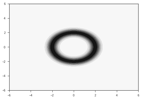
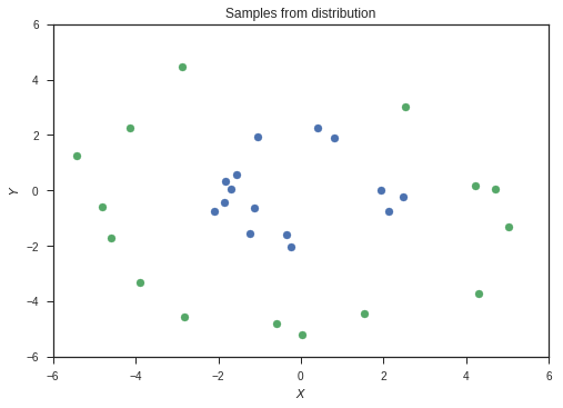
Our input is going to be a vector of size 2. The task is to classify this input into two classes. The two classes are given by two probability distributions over the 2D plane as shown below. They are radial gaussians with different means. The dataset which we use for training will be sampled from these distributions.
def probab(x,y,R = 2,sigma=0.5):
  """2D Radial gaussian distribution."""
  r = np.sqrt(x**2 + y**2)
  p = np.exp(-(r-R)**2/sigma**2)
  return p
# contour plot of distribution
R1=2
R2=5
xr = np.linspace(-6,6,1000)
x,y = np.meshgrid(xr,xr)
p1 = probab(x,y, R = R1)
p2 = probab(x,y,R = R2)
plt.contourf(x,y,p1)
plt.show()
plt.contourf(x,y,p2)
plt.show()
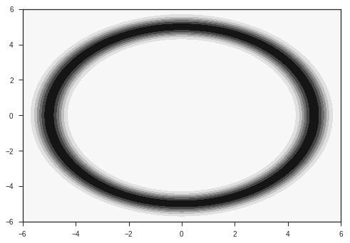
These distributions are the ones from which we will sample our data. In reality, we will have access to only our the sampled data, and won’t have knowledge of these distributions. Also, most of the data in the real world won’t simply be 2 dimensional. Images for example are data points in very high dimensional space, with around 1000 independent dimensions. Keep these two points in mind while following this example.
def sample2d(x,y,p,samples=100):
  """Sample a 2D distribution given by p. The range of values of the two
  variables are given in x and y."""

  # first sample along x
  px = np.sum(p,axis=1) # distribution in x
  px = px/np.sum(px) # normalize

  # get x sample indices
  x_samples_ind = np.random.choice(np.arange(x.shape[0]),samples,p=px)

  # sample along y conditioned on x samples
  y_samples_ind = [np.random.choice(np.arange(y.shape[0]),
                                    p=p[x_ind]/np.sum(p[x_ind]))
                   for x_ind in x_samples_ind]

  # get values
  x_s = [x[i] for i in x_samples_ind]
  y_s = [y[i] for i in y_samples_ind]

  # scatter plot samples
  plt.scatter(x_s, y_s)
  plt.xlim([min(x),max(x)])
  plt.ylim([min(y),max(y)])
  plt.xlabel("$$X$$")
  plt.ylabel("$$Y$$")
  plt.title("Samples from distribution")

  s = np.stack((np.array(x_s),np.array(y_s)))

  return s.T.reshape((-1,2))
samples1 = sample2d(xr,xr,p1,500)
samples2 = sample2d(xr,xr,p2,500)
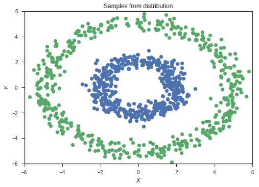
This is our set of sampled data. The colours represent the classes of the two sets of data.
#print(samples1)
#print(samples2)
from keras.layers import *
from keras.models import *
from livelossplot import PlotLossesKeras
The model
The neural network which we are building is a very small one. It has 3 hidden layers, with tanh activations and an output layer with a softmax activation. The softmax activation is defined as follows:
\[\begin{equation} y_i = \frac{e^{z_i}}{\sum_{j=0}^N e^{z_j}} \end{equation}\]Where \(y_i\) represents the \(i^{th}\) element of the output vector. This is the output activation we use for classification tasks, as the values of the output can be interpreted as class probabilities. The loss function to use for classification tasks is called the cross entropy loss. The loss for binary classification is as follows:
\[\begin{equation} −(ylog(p)+(1−y)log(1−p)) \end{equation}\]Where \(y\) is the binary label of the datapoint, and \(p\) is the probability for the input being in that class predicted by our model. The derivations of these activations and losses require probability and information theory concepts, which we won’t get into here.
The first layer has an output of size 4, while the other two have an output of size 2.
inp = Input((2,))

t = Dense(4,activation='tanh')(inp)
layer1 = Dense(2 ,activation='tanh')(t)
layer2 = Dense(2 ,activation='tanh')(layer1)
presoftmax = Dense(2)(layer2)
out = Activation('softmax')(presoftmax)

model = Model(inputs=inp,outputs=out)
model.compile(loss='categorical_crossentropy',optimizer='adam',metrics=['acc'])
print(model.summary())
_________________________________________________________________
Layer (type)                 Output Shape              Param #
=================================================================
input_2 (InputLayer)         (None, 2)                 0
_________________________________________________________________
dense_5 (Dense)              (None, 4)                 12
_________________________________________________________________
dense_6 (Dense)              (None, 2)                 10
_________________________________________________________________
dense_7 (Dense)              (None, 2)                 6
_________________________________________________________________
dense_8 (Dense)              (None, 2)                 6
_________________________________________________________________
activation_2 (Activation)    (None, 2)                 0
=================================================================
Total params: 34
Trainable params: 34
Non-trainable params: 0
_________________________________________________________________
None
train_data = np.concatenate((samples1,samples2))
l1 = np.array([1,0])
l2 = np.array([0,1])
labels = np.concatenate((np.tile(l1,(samples1.shape[0],1)),np.tile(l2,(samples2.shape[0],1))))
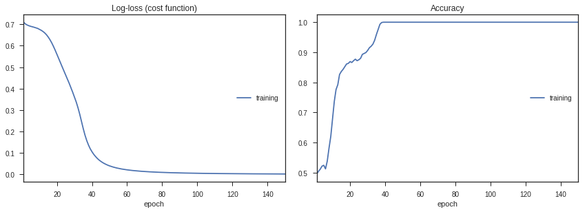
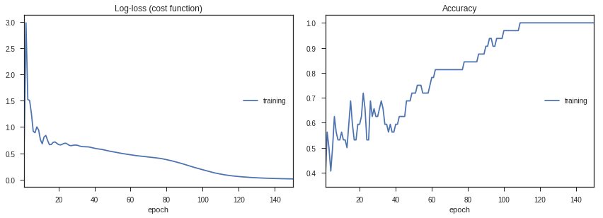
Let’s go ahead and train the model, and look at how the loss and accuracy change with time.
history = model.fit(train_data,labels,epochs=150,callbacks=[PlotLossesKeras(dynamic_x_axis=False)])
def plotModelOut(x,y,model):
  grid = np.stack((x,y))
  grid = grid.T.reshape(-1,2)
  outs = model.predict(grid)
  y1 = outs.T[0].reshape(x.shape[0],x.shape[0])
  plt.contourf(x,y,y1)
  plt.show()
def plotModelGrid(x,y,model=None):
  grid = np.stack((x,y))
  grid = grid.T.reshape(-1,2)

  x_coords = grid.T[0]
  y_coords = grid.T[1]
  class1 = grid[np.where(x_coords**2+y_coords**2>((R1+R2)/2)**2)]
  class2 = grid[np.where(x_coords**2+y_coords**2<=((R1+R2)/2)**2)]

  if model != None:
    outs1 = model.predict(class1)
    outs2 = model.predict(class2)
  else:
    outs1 = class1
    outs2 = class2


  c1 = class1.shape[0]
  x1 = outs1.T[0]
  y1 = outs1.T[1]

  c2 = class2.shape[0]
  x2 = outs2.T[0]
  y2 = outs2.T[1]

  plt.scatter(x2,y2,s=0.05)
  plt.scatter(x1,y1,s=0.05)
  plt.show()
lay1 = Model(inputs=inp,outputs=layer1)
lay2 = Model(inputs=inp,outputs=layer2)
presoft = Model(inputs=inp,outputs=presoftmax)
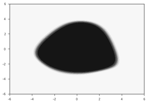
Let’s plot the first component of the output for each point on the x-y plane. This is basically the model’s prediction of the probability of the point belonging to the first class ( the gaussian with smaller radius ).
plotModelOut(x,y,model)
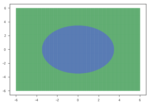
Let’s look at the maps of the hidden layers. The following is the input we give to the model:
plotModelGrid(x,y)
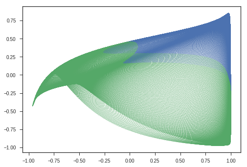
The second layer maps the points with the corresponding colour to the following points:
plotModelGrid(x,y,lay1)
The third layer as follows:
plotModelGrid(x,y,lay2)
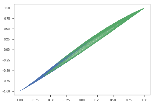
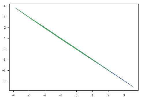
And the output just before applying a softmax looks like this:
plotModelGrid(x,y,presoft)
Outliers and overfitting
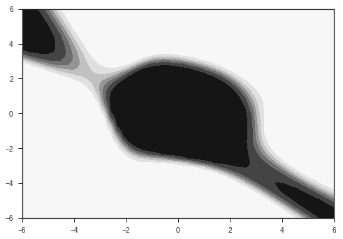
If we have too few samples, and too big a network, the model is extremely sensitive to outliers. This means that the model will try its best to accomodate all the datapoints, which are few in number, and will overfit these points. This is possible because the large number of parameters in the network give it a lot of flexibility.
inp2 = Input((2,))

te = Dense(1000,activation='tanh')(inp2)
te = Dense(1000,activation='tanh')(te)
te = Dense(1000,activation='tanh')(te)
out2 = Dense(2,activation='softmax')(te)

model2 = Model(inputs=inp2,outputs=out2)
model2.compile(loss='categorical_crossentropy',optimizer='adam',metrics=['acc'])
print(model2.summary())
_________________________________________________________________
Layer (type)                 Output Shape              Param #
=================================================================
input_4 (InputLayer)         (None, 2)                 0
_________________________________________________________________
dense_13 (Dense)             (None, 1000)              3000
_________________________________________________________________
dense_14 (Dense)             (None, 1000)              1001000
_________________________________________________________________
dense_15 (Dense)             (None, 1000)              1001000
_________________________________________________________________
dense_16 (Dense)             (None, 2)                 2002
=================================================================
Total params: 2,007,002
Trainable params: 2,007,002
Non-trainable params: 0
_________________________________________________________________
None
samples1_2 = sample2d(xr,xr,p1,15)
samples2_2 = sample2d(xr,xr,p2,15)
train_data2 = np.concatenate((samples1_2,samples2_2,[[-5,5],[5,-5]]))
labels2 = np.concatenate((np.tile(l1,(samples1_2.shape[0],1)),np.tile(l2,(samples2_2.shape[0],1)),np.array([[1,0],[1,0]])))
#plt.scatter([-6],[6],color='blue')
history = model2.fit(train_data2,labels2,epochs=150,callbacks=[PlotLossesKeras(dynamic_x_axis=False)])
h=np.linspace(-6,6,50)
x_, y_ = np.meshgrid(h,h)
plotModelOut(x_,y_,model2)
Linear Algebra Intuition
What does Multiplying a Matrix with a Column Vector do?
Lets assume we have a matrix \(\boldsymbol{A}\) of size \(N*N\) and a column vector \(\boldsymbol{x}\) of size \(N*1\).
\[\begin{equation} y = Ax \end{equation}\]Let’s assume \(A\) is a \(3*3\) Matrix with its entries as follows,
\[\begin{equation} A = \begin{bmatrix} a_1 & a_2 & a_3 \\ b_1 & b_2 & b_3 \\ c_1 & c_2 & c_3 \end{bmatrix} \end{equation}\]and \(x\) to be a column vector (\(3*1\)) \(\begin{equation} x = \begin{bmatrix} x_1 \\ x_2 \\ x_3 \end{bmatrix} \end{equation}\)
Now lets multiply them ans see the resulting output vector,
\[\begin{equation} y = Ax = \begin{bmatrix} a_1 & a_2 & a_3 \\ b_1 & b_2 & b_3 \\ c_1 & c_2 & c_3 \end{bmatrix} \begin{bmatrix} x_1 \\ x_2 \\ x_3 \end{bmatrix} = \begin{bmatrix} a_1x_1 + a_2x_2 + a_3x_3 \\ b_1x_1 + b_2x_2 + b_3x_3 \\ c_1x_1 + c_2x_2 + c_3x_3 \end{bmatrix} \\ = \begin{bmatrix} x_1 \begin{pmatrix} a_1 \\ b_1 \\ c_1 \end{pmatrix} + x_2 \begin{pmatrix} a_2 \\ b_2 \\ c_2 \end{pmatrix} + x_3 \begin{pmatrix} a_3 \\ b_3 \\ c_3 \end{pmatrix} \end{bmatrix} \end{equation}\]So multiplying a matrix with a column vector returns a vector which is a linear combination of its column vectors ( as shown above ).
- \(C(A) =\) It denotes the column space of the matrix \(A\). Column space is the span of all the column vectors of Matrix \(A\).
Intuitively, what does it do?
def transform(A, x, y, bias = ([0,0])):
  '''
  Parameters
  ----------
  A : Matrix that transforms the space
  x: x_coordinates
  y: y_coordinates
  bias: Bias vector to be added

  Returns
  -------
  y_transformed: The transformed space, ([x_trans, y_trans])
  max_value: The maximum value of the distorted + input space
  '''
  x_matrix = np.vstack((x, y))
  y_transformed = (A.dot(x_matrix).T + bias).T
  max_value = np.hstack((x_matrix, y_transformed)).max()
  return y_transformed, max_value
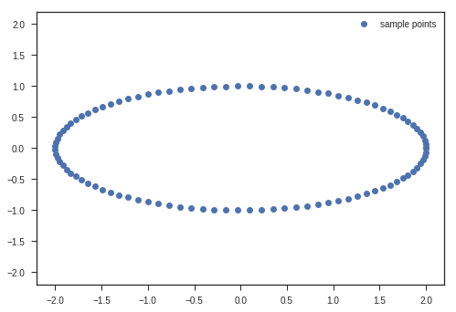
We will show the transformations that matrix multiplication does using an ellipse or a circle. Remember the parametric coordinates of an ellipse or circle?
Parametric Equations of an Ellipse
\[\begin{equation} x = acos(\theta)\\ y = bsin(\theta)\\ \theta\ \epsilon\ [0,2\pi] \end{equation}\]We will use this to plot an ellipse and apply transformations to these coordinates and see the transforms and try to gain intuitions.
t = np.linspace(0, 2*np.pi, 100)

x_c = 2*np.cos(t)
y_c = np.sin(t)
x_matrix = np.vstack((x_c, y_c))
max_value = x_matrix.max()
plt.plot(x_c, y_c, 'o', label = 'sample points')
plt.legend(loc = 'best')
plt.xlim(-1.1*max_value, 1.1*max_value)
plt.ylim(-1.1*max_value, 1.1*max_value)
plt.show()
Lets define a 2-D Matrix A
\[\begin{equation} A = \begin{bmatrix} cos\theta & -sin\theta \\ sin\theta & cos\theta \end{bmatrix} \end{equation}\]Remember distantly what this matrix does?
Its a Rotation Matrix, which rotates the space without scaling the space. We will see the meanings of these terms shortly.
\[\begin{equation} Ax = \begin{bmatrix} cos\theta & -sin\theta \\ sin\theta & cos\theta \end{bmatrix} \begin{bmatrix} x \\ y \end{bmatrix} = \begin{bmatrix} xcos\theta - ysin\theta \\ xsin\theta + ycos\theta \end{bmatrix} = \begin{bmatrix} x^{'} \\ y^{'} \end{bmatrix} \end{equation}\]Whats is the determinant of this Rotation Matrix??
\[\begin{equation} |A| = \begin{vmatrix} cos\theta & -sin\theta \\ sin\theta & cos\theta \end{vmatrix} = cos^{2}\theta + sin^{2}\theta = 1 \end{equation}\]Determinants are related to the volume change during matrix transformation.
-
| A | = 1 would mean that the volume of any closed surface in the space is conserved. The distortion caused by matrix in the space is preserving volume. No closed surface expands or contracts in this transform.
-
| A | > 1 would mean that the volume of any closed surface in space increases.
-
| A | = 0 would mean that the closed surface volume reduces to 0.

This image describes the why this matrix is called Rotation matrix in 2D.
If the input column vector \(x\) is taken to represent coordinates of a point in 2D space, then after doing the transformation ( $(i.e)$ multiplying with matrix \(A\) ),
We get the rotated point represented as \([x^{'}, y^{'}]\) in this image.
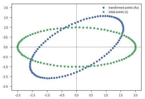
Now we have analysed this matrix transformation for one point. What will happen to a set of points in 2-D space?
theta = np.pi/4
A = np.array([[np.cos(theta), -np.sin(theta)],
              [np.sin(theta), np.cos(theta)]])
y_matrix, max_value = transform(A, x_c, y_c)
plt.plot(y_matrix[0], y_matrix[1], 'o', label = 'transformed points (Ax)')
plt.plot(x_c, y_c,'o', label = 'initial points (x)')
plt.legend(loc = 'best')
plt.xlim(-1.1*max_value, 1.1*max_value)
plt.ylim(-1.1*max_value, 1.1*max_value)
plt.axvline(linewidth=0.5, color = 'k')
plt.axhline(linewidth=0.5, color = 'k')
plt.show()
Observations:
- Entire Ellipse ( Represented in blue ) is rotated with respect to the initial ellipse ( green one ) by the angle \(\theta\) we specified the program.
Inferences:
- This kind of matrix rotate the space. ( If only rotation is desired, keep the determinant 1 )
t = np.linspace(0, 2*np.pi, 100)

x_c = np.cos(t)
y_c = np.sin(t)
x_matrix = np.vstack((x_c, y_c))
max_value = x_matrix.max()
plt.plot(x_c, y_c, 'o', label = 'sample points')
plt.legend(loc = 'best')
plt.xlim(-1.1*max_value, 1.1*max_value)
plt.ylim(-1.1*max_value, 1.1*max_value)
plt.axvline(linewidth=0.5, color = 'k')
plt.axhline(linewidth=0.5, color = 'k')
plt.show()
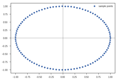
Now, lets take this matrix and study its transform abilities.
\[\begin{equation} A = \begin{bmatrix} 2 & 0 \\ 0 & 1 \end{bmatrix} \end{equation}\]Whats the determinant of this matrix?
\[\begin{equation} |A| = \begin{vmatrix} 2 & 0 \\ 0 & 1 \end{vmatrix} = 2 \end{equation}\]
\(\begin{equation}
Ax =
\begin{bmatrix}
2 & 0 \\
0 & 1
\end{bmatrix}
\begin{bmatrix}
x \\
y
\end{bmatrix} =
\begin{bmatrix}
2x \\
y
\end{bmatrix}
\end{equation}\)
What does this mean?
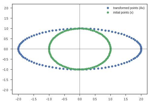
\[\begin{equation} \begin{bmatrix} x \\ y \end{bmatrix} \longrightarrow \begin{bmatrix} 2x \\ y \end{bmatrix} \end{equation}\]This streches the space along x direction, preserving y direction.
Eigen Decomposition
An Eigenvector of a square matrix \(\boldsymbol{A}\) is a non-zero vector \(\boldsymbol{v}\) such that transformation by \(\boldsymbol{A}\) (multiplication by \(\boldsymbol{A}\)) only scales the vector \(\boldsymbol{v}\) by a factor \(\boldsymbol{\lambda}\) which is its ** EigenValue **.
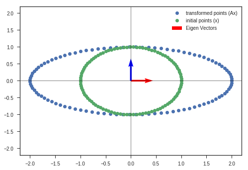
\[\begin{equation} \boldsymbol{A}v = \lambda v \end{equation}\]So, if we find eigenvectors of matrix \(A\), we can say that those directions are the directions that will be only scaled by the transformation by this matrix ( scaled by its eigenvalue ). All the other directions other than eigenvector directions, will be both scaled and rotated, to maintain continuity of the transformation.
If \(\boldsymbol{v}\) is an eigenvector of \(\boldsymbol{A}\), and has an eigenvalue \(\lambda\), whats the eigenvalue of \(c\boldsymbol{v}\), c is a constant?
Its also \(\lambda\) right? So we use unit normalized eigenvectors.
Suppose matrix \(\boldsymbol{A}\) has \(n\) independent eigenvectors, { \(v^{(1)}, v^{(2)}, v^{(3)}, ....., v^{(n)}\) } with its corresponding eigenvalues, { \(\lambda_{1}, \lambda_{2}, ......, \lambda_{n}\) }.
Then, we can concatenate all the eigenvectors into a single matrix called \(\boldsymbol{V}\), which can be represented as
\[\begin{equation} \boldsymbol{V} = \begin{bmatrix} \vdots & \vdots & \vdots & \vdots \\ v^{(1)} & v^{(2)} & \cdots & v^{(n)}\\ \vdots & \vdots & \vdots & \vdots \end{bmatrix}_{n\times n} \end{equation}\]We can define a diagonal matrix, where each diagonal entry is \(\lambda_{i}\) corresponsing to \(v^{(i)}\).
\[\begin{equation} diag(\lambda) = \begin{pmatrix} \lambda_{1}\\ &\lambda_{2}\\ && \lambda_{3}\\ &&& \cdots\\ &&&& \lambda_{n} \end{pmatrix}_{n\times n} \end{equation}\]Then matrix \(\boldsymbol{A}\) can be reconstructed from these matrices \({V}\) and \({diag(\lambda)}\) using eigendecomposition of A, which is given by,
\[\begin{equation} {A} = {V}diag{(\lambda)}{V}^{-1} \end{equation}\]Whats the use of this???
- We can construct a matrix with specific eigenvectors and eigenvalues that allows us to stretch the space in desired directions.
- We can design specific matrices that can distort the space in such a way that data becomes easily separable so that our classifier can separate the data easily. Now you can understand the point of doing all this !!!
We want to create a matrix that can distort the space in such a way that we want our data to get sepatated.
- Neural Nets distort the input data in high dimentional space using these matrix multiplications, ( apply activations in middle ), until the data becomes linearly separable.
- These distortions can be analysed by eigendecomposition and singular value decomposition of weight matrices of the layers of deep neural nets.
A = np.array([[2,0],
              [0,1]])
y_matrix, max_value = transform(A, x_c, y_c)
plt.plot(y_matrix[0], y_matrix[1], 'o', label = 'transformed points (Ax)')
plt.plot(x_c, y_c,'o', label = 'initial points (x)')
plt.legend(loc = 'best')
plt.xlim(-1.1*max_value, 1.1*max_value)
plt.ylim(-1.1*max_value, 1.1*max_value)
plt.axvline(linewidth=0.5, color = 'k')
plt.axhline(linewidth=0.5, color = 'k')
plt.show()
def eigen_decomposition(A, x, y, scale_by_eigen = False, bias = np.array([0,0])):
  y_matrix, max_value = transform(A, x, y, bias)
  W, V = np.linalg.eig(A)
  SCALE = 10
  # print (V.shape, W.shape)
  if scale_by_eigen:
    V[:,range(len(W))]*= W   # Multiplying the EigenVector with Eigenvalue
  no_of_points =  len(V[:,0])
  plt.quiver(np.zeros(no_of_points),np.zeros(no_of_points)  , V[0], V[1],color = ['r', 'b'], scale = SCALE, label = 'Eigen Vectors')
  plt.plot(y_matrix[0], y_matrix[1], 'o', label = 'transformed points (Ax)')
  plt.plot(x, y,'o', label = 'initialnp.array(bias) points (x)')
  plt.xlim(-1.1*max_value, 1.1*max_value)
  plt.ylim(-1.1*max_value, 1.1*max_value)
  plt.axvline(linewidth=0.5, color = 'k')
  plt.axhline(linewidth=0.5, color = 'k')
  plt.quiver([0], [0], bias[0], bias[1], scale = 21, label = 'Bias Vector')
  plt.legend(loc = 'best')
  return W, V, y_matrix
w_1, v_1, y_matrix_1 = eigen_decomposition(A, x_c, y_c)
A = np.array([[6,2],
              [3,2]])
w_2, v_2, y_matrix_2 = eigen_decomposition(A, x_c, y_c)
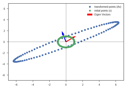
Obseravtions:
- The vectors near to eigenvectors do not rotate that much. They get scaled by the eigenvalue ( if its an eigenvector, else a small rotation is present ).
- Vectors that are far away from either of the eigenvectors are severly rotated and scaled. ( Maintain the continuity of the figure )
- Volume has increased greater than the initial circle, which indicates that the determinant of the matrix is greater than 1.
bias = [0,4]
w_2b, v_2b, y_matrix_2b = eigen_decomposition(A, x_c, y_c, bias = bias)
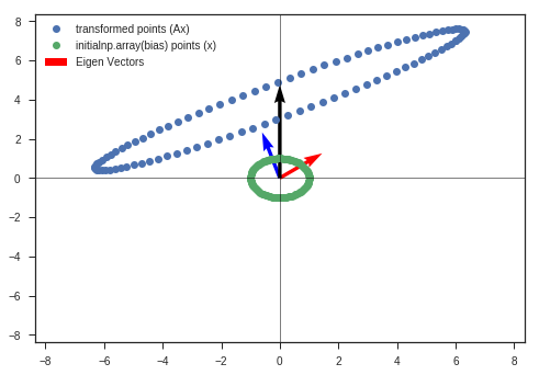
Observations:
- Other than other observations ( listed in the previous plot ), we can see the bias has just shifted the distorted figure along that direction ( bias vector’s direction ).
So we now know why bias is needed
This is because, if bias is not added we are restricted with origin as center. It is similar to
\[\begin{equation} y = mx + b \end{equation}\]where b acts as a bias. If \(b = 0\), we will be restricted to only use lines which pass through origin.
\[\begin{equation} y = mx \end{equation}\]So addition of bias gives extra freedom to move anywhere in the space ( translation ) and multiplying with the weight matrix enables the model to distort, scale, or rotate the space ( with center at origin ) the space.
So Neural Net basicaly traanslates ( due to the bias ), distorts data points by scaling and rotating them ( weights ) in hyperdimentional space, with an aim to find a transformation to make the data linearly separable at the end.
# What if determinant is 0?
A = np.array([[3,2],
              [3,2]])
w_3, v_3, y_matrix_2 = eigen_decomposition(A, x_c, y_c)
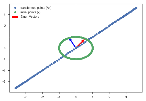
Observation:
- Determinant of the transformation matrix is 0.
- The space is completely contracted along one-dimension, causing it to lose all of its volume.
# What if determinant is < 0?
A_plus = np.array([[6,2],
                   [3,2]])

A_minus = np.array([[-6,-2],
                   [3,2]])

x = np.linspace(-1,1,10)
y = x**2
w_3, v_3, y_matrix_3 = eigen_decomposition(A_plus, x, y)
plt.show()
w_4, v_4, y_matrix_4 = eigen_decomposition(A_minus, x, y)
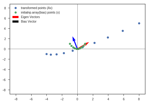
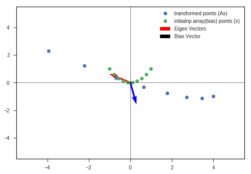
When Determinant is less than zero we get a reflection about y axis but the deformation is same ( except the reflection )
Enough of theory! Lets have an hands on seesion how to implement neural networks!
from keras.datasets import mnist
(train_images, train_labels), (test_images, test_labels) = mnist.load_data()
from keras.utils import to_categorical

print('Training data shape : ', train_images.shape, train_labels.shape)

print('Testing data shape : ', test_images.shape, test_labels.shape)

# Find the unique numbers from the train labels
classes = np.unique(train_labels)
nClasses = len(classes)
print('Total number of outputs : ', nClasses)
print('Output classes : ', classes)

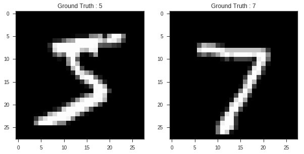
plt.figure(figsize=[10,5])

# Display the first image in training data
plt.subplot(121)
plt.imshow(train_images[0,:,:], cmap='gray')
plt.title("Ground Truth : {}".format(train_labels[0]))

# Display the first image in testing data
plt.subplot(122)
plt.imshow(test_images[0,:,:], cmap='gray')
plt.title("Ground Truth : {}".format(test_labels[0]))
Training data shape :  (60000, 28, 28) (60000,)
Testing data shape :  (10000, 28, 28) (10000,)
Total number of outputs :  10
Output classes :  [0 1 2 3 4 5 6 7 8 9]


Text(0.5,1,'Ground Truth : 7')
# Change from matrix to array of dimension 28x28 to array of dimention 784
dimData = np.prod(train_images.shape[1:])
train_data = train_images.reshape(train_images.shape[0], dimData)
test_data = test_images.reshape(test_images.shape[0], dimData)
# Change to float datatype
train_data = train_data.astype('float32')
test_data = test_data.astype('float32')

# Scale the data to lie between 0 to 1
train_data /= 255
test_data /= 255
# Change the labels from integer to categorical data
train_labels_one_hot = to_categorical(train_labels)
test_labels_one_hot = to_categorical(test_labels)

# Display the change for category label using one-hot encoding
print('Original label 0 : ', train_labels[0])
print('After conversion to categorical ( one-hot ) : ', train_labels_one_hot[0])
Original label 0 :  5
After conversion to categorical ( one-hot ) :  [0. 0. 0. 0. 0. 1. 0. 0. 0. 0.]
from keras.models import Sequential
from keras.layers import Dense

model = Sequential()
model.add(Dense(512, activation='relu', input_shape=(dimData,)))
model.add(Dense(512, activation='relu'))
model.add(Dense(nClasses, activation='softmax'))
model.compile(optimizer='rmsprop', loss='categorical_crossentropy', metrics=['accuracy'])
history = model.fit(train_data, train_labels_one_hot, batch_size=256, epochs=20, verbose=1,
                   validation_data=(test_data, test_labels_one_hot))
Train on 60000 samples, validate on 10000 samples
Epoch 1/20
60000/60000 [==============================] - 5s 91us/step - loss: 1.0680 - acc: 0.6747 - val_loss: 0.5387 - val_acc: 0.8440
Epoch 2/20
60000/60000 [==============================] - 6s 103us/step - loss: 0.4464 - acc: 0.8695 - val_loss: 0.3897 - val_acc: 0.8838
Epoch 3/20
60000/60000 [==============================] - 6s 104us/step - loss: 0.3504 - acc: 0.8975 - val_loss: 0.3262 - val_acc: 0.9030
Epoch 4/20
13568/60000 [=====>........................] - ETA: 4s - loss: 0.3212 - acc: 0.908260000/60000 [==============================] - 6s 105us/step - loss: 0.3030 - acc: 0.9112 - val_loss: 0.2947 - val_acc: 0.9089
Epoch 5/20
60000/60000 [==============================] - 6s 105us/step - loss: 0.2643 - acc: 0.9220 - val_loss: 0.2420 - val_acc: 0.9299
Epoch 6/20
60000/60000 [==============================] - 6s 105us/step - loss: 0.2319 - acc: 0.9311 - val_loss: 0.2284 - val_acc: 0.9311
Epoch 7/20
30976/60000 [==============>...............] - ETA: 2s - loss: 0.2073 - acc: 0.938860000/60000 [==============================] - 6s 106us/step - loss: 0.2039 - acc: 0.9396 - val_loss: 0.2231 - val_acc: 0.9314
Epoch 8/20
60000/60000 [==============================] - 6s 104us/step - loss: 0.1785 - acc: 0.9468 - val_loss: 0.1728 - val_acc: 0.9491
Epoch 9/20
60000/60000 [==============================] - 6s 103us/step - loss: 0.1581 - acc: 0.9523 - val_loss: 0.1768 - val_acc: 0.9458
Epoch 10/20
38656/60000 [==================>...........] - ETA: 2s - loss: 0.1424 - acc: 0.956960000/60000 [==============================] - 6s 105us/step - loss: 0.1405 - acc: 0.9571 - val_loss: 0.1348 - val_acc: 0.9581
Epoch 11/20
60000/60000 [==============================] - 6s 103us/step - loss: 0.1260 - acc: 0.9627 - val_loss: 0.1439 - val_acc: 0.9541
Epoch 12/20
60000/60000 [==============================] - 6s 104us/step - loss: 0.1137 - acc: 0.9662 - val_loss: 0.1407 - val_acc: 0.9564
Epoch 13/20
39936/60000 [==================>...........] - ETA: 1s - loss: 0.1070 - acc: 0.968560000/60000 [==============================] - 6s 104us/step - loss: 0.1032 - acc: 0.9695 - val_loss: 0.1162 - val_acc: 0.9646
Epoch 14/20
60000/60000 [==============================] - 6s 103us/step - loss: 0.0939 - acc: 0.9714 - val_loss: 0.1147 - val_acc: 0.9663
Epoch 15/20
60000/60000 [==============================] - 6s 104us/step - loss: 0.0854 - acc: 0.9745 - val_loss: 0.1040 - val_acc: 0.9677
Epoch 16/20
42752/60000 [====================>.........] - ETA: 1s - loss: 0.0793 - acc: 0.976760000/60000 [==============================] - 6s 104us/step - loss: 0.0782 - acc: 0.9762 - val_loss: 0.0975 - val_acc: 0.9711
Epoch 17/20
60000/60000 [==============================] - 6s 103us/step - loss: 0.0724 - acc: 0.9779 - val_loss: 0.0920 - val_acc: 0.9710
Epoch 18/20
60000/60000 [==============================] - 6s 103us/step - loss: 0.0663 - acc: 0.9799 - val_loss: 0.0840 - val_acc: 0.9751
Epoch 19/20
43008/60000 [====================>.........] - ETA: 1s - loss: 0.0605 - acc: 0.981360000/60000 [==============================] - 6s 105us/step - loss: 0.0619 - acc: 0.9810 - val_loss: 0.0831 - val_acc: 0.9757
Epoch 20/20
60000/60000 [==============================] - 6s 103us/step - loss: 0.0564 - acc: 0.9833 - val_loss: 0.0912 - val_acc: 0.9703
[test_loss, test_acc] = model.evaluate(test_data, test_labels_one_hot)
print("Evaluation result on Test Data : Loss = {}, accuracy = {}".format(test_loss, test_acc))
10000/10000 [==============================] - 1s 59us/step
Evaluation result on Test Data : Loss = 0.09124259161902591, accuracy = 0.9703
#Plot the Loss Curves
plt.figure(figsize=[8,6])
plt.plot(history.history['loss'],'r',linewidth=3.0)
plt.plot(history.history['val_loss'],'b',linewidth=3.0)
plt.legend(['Training loss', 'Validation Loss'],fontsize=18)
plt.xlabel('Epochs ',fontsize=16)
plt.ylabel('Loss',fontsize=16)
plt.title('Loss Curves',fontsize=16)

#Plot the Accuracy Curves
plt.figure(figsize=[8,6])
plt.plot(history.history['acc'],'r',linewidth=3.0)
plt.plot(history.history['val_acc'],'b',linewidth=3.0)
plt.legend(['Training Accuracy', 'Validation Accuracy'],fontsize=18)
plt.xlabel('Epochs ',fontsize=16)
plt.ylabel('Accuracy',fontsize=16)
plt.title('Accuracy Curves',fontsize=16)
Text(0.5,1,'Accuracy Curves')
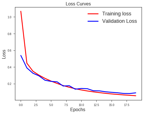
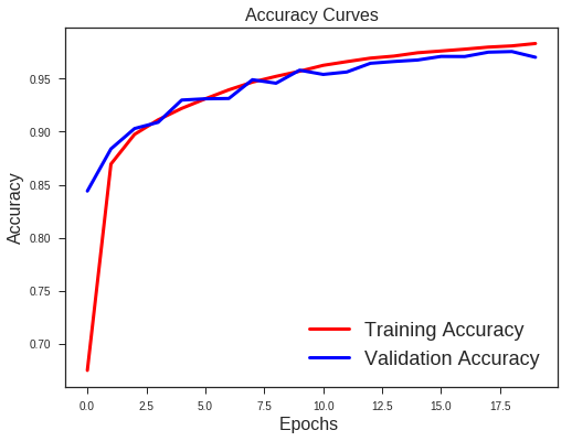
There is a clear sign of Overfitting. Why do you think so?
Carefully see the Validation loss and Training loss curve. Validation loss decreases and then it gradually increases. This means that model is memorising the dataset, though in this case accuracy is much higher.
How to combat this??
Use Regularization !
from keras.layers import Dropout

model_reg = Sequential()
model_reg.add(Dense(512, activation='relu', input_shape=(dimData,)))
model_reg.add(Dropout(0.5))
model_reg.add(Dense(512, activation='relu'))
model_reg.add(Dropout(0.5))
model_reg.add(Dense(nClasses, activation='softmax'))
model_reg.compile(optimizer='rmsprop', loss='categorical_crossentropy', metrics=['accuracy'])
history_reg = model_reg.fit(train_data, train_labels_one_hot, batch_size=256, epochs=20, verbose=1,
                            validation_data=(test_data, test_labels_one_hot))

#Plot the Loss Curves
plt.figure(figsize=[8,6])
plt.plot(history_reg.history['loss'],'r',linewidth=3.0)
plt.plot(history_reg.history['val_loss'],'b',linewidth=3.0)
plt.legend(['Training loss', 'Validation Loss'],fontsize=18)
plt.xlabel('Epochs ',fontsize=16)
plt.ylabel('Loss',fontsize=16)
plt.title('Loss Curves',fontsize=16)

#Plot the Accuracy Curves
plt.figure(figsize=[8,6])
plt.plot(history_reg.history['acc'],'r',linewidth=3.0)
plt.plot(history_reg.history['val_acc'],'b',linewidth=3.0)
plt.legend(['Training Accuracy', 'Validation Accuracy'],fontsize=18)
plt.xlabel('Epochs ',fontsize=16)
plt.ylabel('Accuracy',fontsize=16)
plt.title('Accuracy Curves',fontsize=16)
Train on 60000 samples, validate on 10000 samples
Epoch 1/20
60000/60000 [==============================] - 6s 106us/step - loss: 0.3708 - acc: 0.8850 - val_loss: 0.1496 - val_acc: 0.9529
Epoch 2/20
60000/60000 [==============================] - 7s 117us/step - loss: 0.1690 - acc: 0.9491 - val_loss: 0.0993 - val_acc: 0.9688
Epoch 3/20
60000/60000 [==============================] - 7s 118us/step - loss: 0.1310 - acc: 0.9607 - val_loss: 0.0904 - val_acc: 0.9727
Epoch 4/20
 1280/60000 [..............................] - ETA: 6s - loss: 0.1252 - acc: 0.964160000/60000 [==============================] - 7s 119us/step - loss: 0.1094 - acc: 0.9679 - val_loss: 0.0852 - val_acc: 0.9760
Epoch 5/20
60000/60000 [==============================] - 7s 119us/step - loss: 0.0974 - acc: 0.9711 - val_loss: 0.0920 - val_acc: 0.9737
Epoch 6/20
60000/60000 [==============================] - 7s 119us/step - loss: 0.0866 - acc: 0.9750 - val_loss: 0.0783 - val_acc: 0.9784
Epoch 7/20
21760/60000 [=========>....................] - ETA: 4s - loss: 0.0776 - acc: 0.977560000/60000 [==============================] - 7s 118us/step - loss: 0.0803 - acc: 0.9766 - val_loss: 0.0714 - val_acc: 0.9803
Epoch 8/20
60000/60000 [==============================] - 7s 118us/step - loss: 0.0789 - acc: 0.9768 - val_loss: 0.0688 - val_acc: 0.9811
Epoch 9/20
60000/60000 [==============================] - 7s 118us/step - loss: 0.0715 - acc: 0.9785 - val_loss: 0.0784 - val_acc: 0.9795
Epoch 10/20
25344/60000 [===========>..................] - ETA: 3s - loss: 0.0629 - acc: 0.981660000/60000 [==============================] - 7s 117us/step - loss: 0.0674 - acc: 0.9803 - val_loss: 0.0740 - val_acc: 0.9794
Epoch 11/20
60000/60000 [==============================] - 7s 118us/step - loss: 0.0648 - acc: 0.9806 - val_loss: 0.0776 - val_acc: 0.9806
Epoch 12/20
60000/60000 [==============================] - 7s 119us/step - loss: 0.0633 - acc: 0.9818 - val_loss: 0.0749 - val_acc: 0.9814
Epoch 13/20
25344/60000 [===========>..................] - ETA: 3s - loss: 0.0593 - acc: 0.982860000/60000 [==============================] - 7s 119us/step - loss: 0.0603 - acc: 0.9828 - val_loss: 0.0735 - val_acc: 0.9835
Epoch 14/20
60000/60000 [==============================] - 7s 119us/step - loss: 0.0579 - acc: 0.9829 - val_loss: 0.0770 - val_acc: 0.9824
Epoch 15/20
60000/60000 [==============================] - 7s 119us/step - loss: 0.0557 - acc: 0.9835 - val_loss: 0.0843 - val_acc: 0.9817
Epoch 16/20
25344/60000 [===========>..................] - ETA: 3s - loss: 0.0526 - acc: 0.984660000/60000 [==============================] - 7s 117us/step - loss: 0.0544 - acc: 0.9843 - val_loss: 0.0769 - val_acc: 0.9819
Epoch 17/20
60000/60000 [==============================] - 7s 117us/step - loss: 0.0546 - acc: 0.9849 - val_loss: 0.0762 - val_acc: 0.9825
Epoch 18/20
60000/60000 [==============================] - 7s 117us/step - loss: 0.0522 - acc: 0.9856 - val_loss: 0.0772 - val_acc: 0.9844
Epoch 19/20
25344/60000 [===========>..................] - ETA: 3s - loss: 0.0485 - acc: 0.986360000/60000 [==============================] - 7s 117us/step - loss: 0.0490 - acc: 0.9858 - val_loss: 0.0758 - val_acc: 0.9826
Epoch 20/20
60000/60000 [==============================] - 7s 117us/step - loss: 0.0488 - acc: 0.9860 - val_loss: 0.0773 - val_acc: 0.9846


Text(0.5,1,'Accuracy Curves')
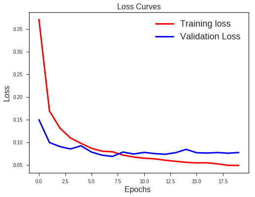
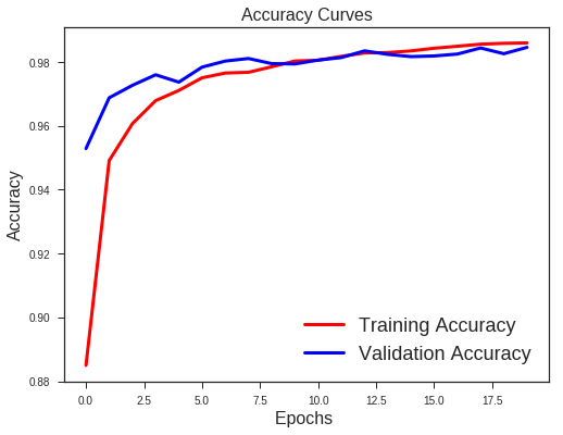
What we note??
- Validation loss is not increasing as it did before.
- Difference between the validation and training accuracy is not that much
This implies better generalisation and can work well on new unseen data samples.
Time to train your own neural network !!!
!pip install matplotlib

from keras.datasets import cifar10
import numpy as np
(train_images, train_labels), (test_images, test_labels)  = cifar10.load_data()
from keras.utils import to_categorical

print('Training data shape : ', train_images.shape, train_labels.shape)

print('Testing data shape : ', test_images.shape, test_labels.shape)

# Find the unique numbers from the train labels
classes = np.unique(train_labels)
nClasses = len(classes)
print('Total number of outputs : ', nClasses)
print('Output classes : ', classes)

plt.figure(figsize=[5,2])

# Display the first image in training data
plt.subplot(121)
plt.imshow(train_images[0,:,:], cmap='gray')
plt.title("Ground Truth : {}".format(train_labels[0]))

# Display the first image in testing data
plt.subplot(122)
plt.imshow(test_images[0,:,:], cmap='gray')
plt.title("Ground Truth : {}".format(test_labels[0]))
# Change from matrix to array of dimension 28x28 to array of dimention 784
dimData = np.prod(train_images.shape[1:])
train_data = train_images.reshape(train_images.shape[0], dimData)
test_data = test_images.reshape(test_images.shape[0], dimData)
# Change to float datatype
train_data = train_data.astype('float32')
test_data = test_data.astype('float32')

# Scale the data to lie between 0 to 1
train_data /= 255
test_data /= 255
# Change the labels from integer to categorical data
train_labels_one_hot = to_categorical(train_labels)
test_labels_one_hot = to_categorical(test_labels)

# Display the change for category label using one-hot encoding
print('Original label 0 : ', train_labels[0])
print('After conversion to categorical ( one-hot ) : ', train_labels_one_hot[0])
Original label 0 :  [6]
After conversion to categorical ( one-hot ) :  [0. 0. 0. 0. 0. 0. 1. 0. 0. 0.]
from keras.models import Sequential
from keras.layers import Dense

model = Sequential()

model.add(Dense(720, activation='sigmoid', input_shape=(dimData,)))
model.add(Dense(720, activation='relu', input_shape=(dimData,)))
model.add(Dense(720, activation='sigmoid', input_shape=(dimData,)))
model.add(Dense(720, activation='relu', input_shape=(dimData,)))
model.add(Dense(720, activation='sigmoid', input_shape=(dimData,)))
model.add(Dense(720, activation='relu', input_shape=(dimData,)))
model.add(Dense(720, activation='sigmoid', input_shape=(dimData,)))
model.add(Dense(720, activation='relu', input_shape=(dimData,)))
model.add(Dense(720, activation='sigmoid', input_shape=(dimData,)))
model.add(Dense(720, activation='relu', input_shape=(dimData,)))
model.add(Dense(720, activation='relu'))
model.add(Dense(nClasses, activation='softmax'))
model.compile(optimizer='rmsprop', loss='categorical_crossentropy', metrics=['accuracy'])
history = model.fit(train_data, train_labels_one_hot, batch_size=256, epochs=20, verbose=1,
                   validation_data=(test_data, test_labels_one_hot))
Train on 50000 samples, validate on 10000 samples
Epoch 1/20
50000/50000 [==============================] - 50s 1ms/step - loss: 2.3366 - acc: 0.0991 - val_loss: 2.3026 - val_acc: 0.1000
Epoch 2/20
50000/50000 [==============================] - 49s 985us/step - loss: 2.3027 - acc: 0.0978 - val_loss: 2.3026 - val_acc: 0.1000
Epoch 3/20
 9472/50000 [====>.........................] - ETA: 37s - loss: 2.3026 - acc: 0.098450000/50000 [==============================] - 49s 985us/step - loss: 2.3027 - acc: 0.0973 - val_loss: 2.3026 - val_acc: 0.1000
Epoch 4/20
50000/50000 [==============================] - 49s 988us/step - loss: 2.3027 - acc: 0.0962 - val_loss: 2.3026 - val_acc: 0.1000
Epoch 5/20
29952/50000 [================>.............] - ETA: 18s - loss: 2.3026 - acc: 0.098050000/50000 [==============================] - 50s 991us/step - loss: 2.3027 - acc: 0.0977 - val_loss: 2.3026 - val_acc: 0.1000
Epoch 6/20
50000/50000 [==============================] - 49s 989us/step - loss: 2.3027 - acc: 0.0980 - val_loss: 2.3026 - val_acc: 0.1000
Epoch 7/20
34560/50000 [===================>..........] - ETA: 14s - loss: 2.3027 - acc: 0.095350000/50000 [==============================] - 49s 986us/step - loss: 2.3027 - acc: 0.0953 - val_loss: 2.3026 - val_acc: 0.1000
Epoch 8/20
50000/50000 [==============================] - 49s 985us/step - loss: 2.3027 - acc: 0.0978 - val_loss: 2.3026 - val_acc: 0.1000
Epoch 9/20
35584/50000 [====================>.........] - ETA: 13s - loss: 2.3027 - acc: 0.098050000/50000 [==============================] - 49s 985us/step - loss: 2.3027 - acc: 0.0967 - val_loss: 2.3026 - val_acc: 0.1000
Epoch 10/20
50000/50000 [==============================] - 49s 986us/step - loss: 2.3027 - acc: 0.0970 - val_loss: 2.3026 - val_acc: 0.1000
Epoch 11/20
35584/50000 [====================>.........] - ETA: 13s - loss: 2.3027 - acc: 0.096950000/50000 [==============================] - 49s 985us/step - loss: 2.3027 - acc: 0.0964 - val_loss: 2.3026 - val_acc: 0.1000
Epoch 12/20
50000/50000 [==============================] - 49s 987us/step - loss: 2.3027 - acc: 0.0971 - val_loss: 2.3026 - val_acc: 0.1000
Epoch 13/20
35584/50000 [====================>.........] - ETA: 13s - loss: 2.3026 - acc: 0.098350000/50000 [==============================] - 49s 989us/step - loss: 2.3027 - acc: 0.0983 - val_loss: 2.3026 - val_acc: 0.1000
Epoch 14/20
25088/50000 [==============>...............] - ETA: 23s - loss: 2.3026 - acc: 0.1005
[test_loss, test_acc] = model.evaluate(test_data, test_labels_one_hot)
print("Evaluation result on Test Data : Loss = {}, accuracy = {}".format(test_loss, test_acc))
10000/10000 [==============================] - 2s 250us/step
Evaluation result on Test Data : Loss = 1.4804802495956422, accuracy = 0.4701
Try to maximize your test accuracy!!! Take it as a challenge. ( Tuning parameters is an art :P )


Leave a Comment