Support Vector Machines and Neural Networks for Image Processing - Part 1

This post forms the first part of the introductory material covered during our sessions on SVMs and Neural Networks. Both posts are slightly more biased towards a probabilistic angle to build intuition.

What are Support Vector Machines?

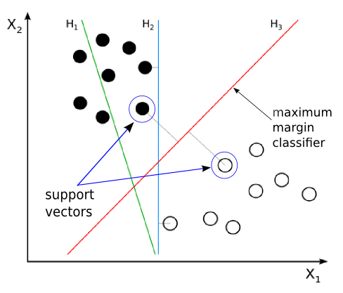
• Given 2 classes as shown in the image, \(H1, H2\) and \(H3\) all represent the possible decision boundaries that can be predicted to be your classifier. Which decision boundary is the preferred one?

• \(H1\) is wrong as it is not separating the classes properly

• Both \(H2\) and \(H3\) separate the classes correctly. What’s the difference between these decision boundaries?

• The problem is that even if the data is linearly separable, we can’t be sure about which line (\(H1, H2, H3\)) the classifier ends up learning. \(SVM\)s were initially born out of the need to answer this question.

The answer to this question is to define an Optimal Separating Hyperplane.

---

What is an Optimal Separating Hyperplane?

It is a surface defined such that the nearest data point to the surface is as far away as possible from it ( as compared to other surfaces ) .

• The nearest data point need not belong to just one class.

• So in the previous image, the line \(H2\) is by definition not a optimal separating hyperplane. This is because, it is not satisfying the “as far away as possible” condition. In fact the data points are very close to the separating hyper plane in this case.

• On the other hand, \(H3\) is optimally separating the data points since the distance from either class’s data points are maximum, and any further change in its position will result in reducing the distance between the one of the nearest data points and the hyperplane.

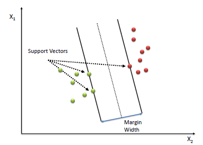
• When you are maximising the distance of the closest points from the separating hyperplane, it basically means that the closest data point from both the classes are at the same distance from the hyper plane.

So the aim of the classifier is to make the margin as large as possible. Now intuitively lets see what such a line means…..

For any linear classifier ( as covered in Linear Regression and Logistic Regression ) we have covered so far, we have seen,

\[\begin{equation} y = \beta_{0} + x_{1}\beta_{1} + x_2\beta_2 + ...... + x_n\beta_n \end{equation}\]

represents the line that acts as a decision boundary in linear classifiers. Where

\(x_1, x_2, ...., x_n\) are the features ( inputs )

and

\(\beta_0\) is the bias and \(\beta_1, \beta_2, ...... \beta_n\) are the weights.

Now for convenience let us define 2 matrices:

\[\begin{equation} \beta = \begin{bmatrix} \beta_1 \\ \beta_2 \\ \vdots \\ \beta_n \end{bmatrix}_{n \times 1} \\ x = \begin{bmatrix} x_1 \\ x_2 \\ \vdots \\ x_n \end{bmatrix}_{n \times 1} \\ \end{equation}\]

Note that,

\[\begin{equation} x^{T}\beta = \begin{bmatrix} x_1 & x_2 & \dots & x_n \end{bmatrix}_{1 \times n} \begin{bmatrix} \beta_1 \\ \beta_2 \\ \vdots \\ \beta_n \end{bmatrix}_{n \times 1} = \sum_{i = 1}^{n}\beta_ix_i \\ y = \beta_0 + x^{T}\beta \end{equation}\]

So all the points satisfying the condition \(y = 0\) represent the decision boundary and the solid black line in the figure. ( Since the image is in 2 dimensions, the equation of the decision boundary reduces to \(y = \beta_0 + \beta_1x\). )

In a normal linear classifier, what would we have done?

If, \(\begin{equation} \beta_0 + x^T\beta < 0 \implies Class\ -1 \\ \beta_0 + x^T\beta > 0 \implies Class\ +1 \end{equation}\) Notice the class encocings

And what exactly do we seek in a SVM?

We want the point to be atleast \(M\) ( Margin ) distance away from the line \(\beta_0 + x^{T}\beta = 0\).

So our optimization problem changes to,

\[\begin{equation} \beta_0 + x_i^T\beta < M \implies y_i = -1 \\ \beta_0 + x_i^T\beta > M \implies y_i = +1 \end{equation}\]

Where \(y_i\) is the class label.

In a single line it can be written as

\[\begin{equation} y_i(\beta_0 + x_i^T\beta) > M \end{equation}\]

This is our constraint. What’s our objective ?

Our objective is to maximize the margin of the classifier. So the optimization unfolds like this,

\[\begin{equation} \max_{\beta_0, \beta, ||\beta|| = 1} M \\ \\ subject\ to\ y_i(\beta_0 + x_i^T\beta) > M\ \forall\ i \end{equation}\]

Assuming that the data is distinctly separated and a nice line can be drawn to separate it.

Solving this optimization problem (We will not go into the details here) we will get \(\beta_0, \beta_{n \times 1}\) which represents the optimal separating hyperplane with maximum margin.

Note that in the way in which we have formulated this optimization problem, we are maximizing the margin without allowing ( strictly ) any data points inside that margin. ( No Tolerence whatsoever )

Solving this optimization problem, we can show that:

• Only the data points on the margin matter when determining the values of \(\beta_0\) and \(\beta_{n\times 1}\).

• Other points which are not on the margin ( which are further away from the margin ) do not affect the solution.

• Vectors ( data points \(x\) ) which are on the margin are called support vectors. They effectively support the margin of the classifier.

!pip install keras
import numpy as np
import scipy
import matplotlib.cm as cm
import matplotlib.pyplot as plt
import os
from random import shuffle
from sklearn.decomposition import PCA
from sklearn.metrics import classification_report
from sklearn.metrics import confusion_matrix
from sklearn.svm import SVC
from sklearn import datasets
import seaborn
from sklearn.datasets import make_classification, make_blobs, make_gaussian_quantiles
seaborn.set(style='ticks')

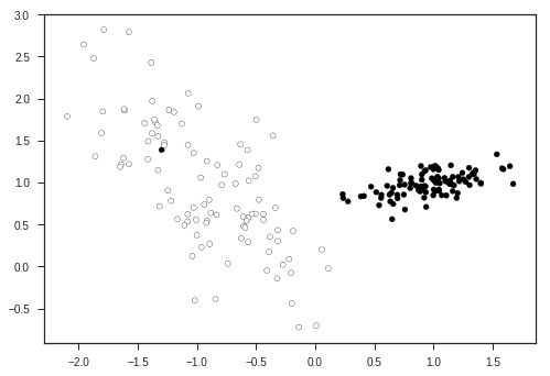
X1, Y1 = make_classification(n_samples = 200, n_features = 2, n_redundant=0, n_informative =2,
                            n_clusters_per_class = 1, class_sep = 1)
plt.scatter(X1[:,0], X1[:,1], marker = 'o', c= (Y1), s = 25, edgecolor = 'k')
plt.show()

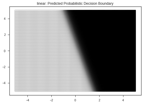
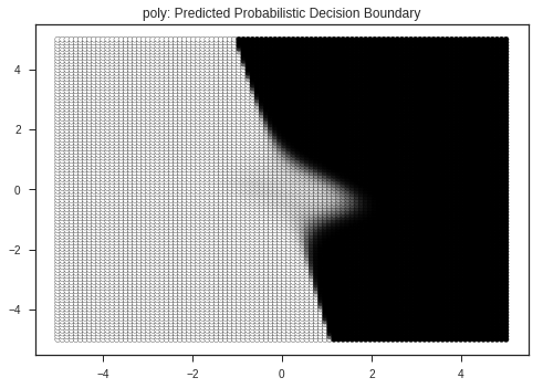
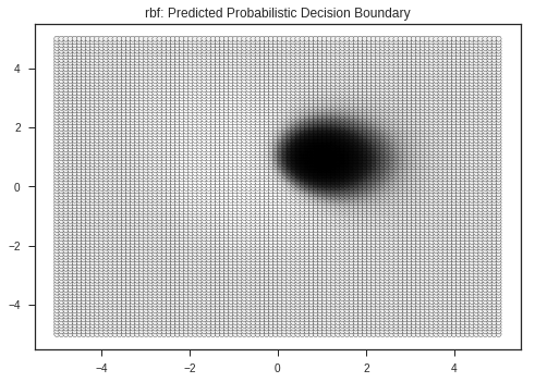
Let’s view the decision boundaries predicted by various kernals ( a kernel is a similarity function with is passed to the SVM function ), here:

• RBF ( Radial Basis Function )
• Linear
• Polynomial

dataset = list(zip(X1, Y1))
shuffle(dataset)
X1, Y1 = list(zip(*dataset))

x_train = X1[:int(0.8*len(X1))]
x_test = X1[int(-0.2*len(X1)):]
y_train = Y1[:int(0.8*len(X1))]
y_test = Y1[int(-0.2*len(X1)):]

kernel_list = ['linear', 'poly', 'rbf']

for idx,kernel in enumerate(kernel_list):
  clf = SVC(gamma = 0.5, kernel = kernel, probability = True)
  clf.fit(x_train, y_train)
  y_pred = clf.predict(x_test)
  print ("Kernel: " + kernel + "'s Report")
  print (classification_report(y_test, y_pred))
  print ("Test Score: \t" + str(np.mean((y_pred == y_test).astype('int'))))
  x = np.linspace(-5, 5, 100)
  xx,yy = np.meshgrid(x,x)
  x_feature = np.vstack((xx.flatten(), yy.flatten())).T
  # print (x_feature.shape)
  y_mesh = clf.predict(x_feature)
  prob_mesh = clf.predict_proba(x_feature)
  prob_mesh_1 =  (prob_mesh.T[1])   # Probability of class 1 (0 means WHITE, 1 means black)
  plt.scatter(xx.flatten(), yy.flatten(), marker = 'o',c = prob_mesh.T[1].flatten(), s = 25, edgecolor = 'k')
  plt.title(kernel + ": Predicted Probabilistic Decision Boundary")
  plt.show()
  #   ax.title(kernel + " : Predicted probabilistic decision boundary")

Kernel: linear's Report
             precision    recall  f1-score   support

          0       0.95      1.00      0.98        20
          1       1.00      0.95      0.97        20

avg / total       0.98      0.97      0.97        40

Test Score: 	0.975

Kernel: poly's Report
             precision    recall  f1-score   support

          0       0.95      1.00      0.98        20
          1       1.00      0.95      0.97        20

avg / total       0.98      0.97      0.97        40

Test Score: 	0.975

Kernel: rbf's Report
             precision    recall  f1-score   support

          0       0.95      1.00      0.98        20
          1       1.00      0.95      0.97        20

avg / total       0.98      0.97      0.97        40

Test Score: 	0.975

clf = SVC(kernel = 'linear')
clf.fit(x_train, y_train)
w = clf.coef_[0]
a = -w[0] / w[1]
xx = np.linspace(-5, 5)
yy = a * xx - (clf.intercept_[0]) / w[1]
margin = 1 / np.sqrt(np.sum(clf.coef_ ** 2))
print ("Margin of the Classifier: " + str(margin))
yy_down = yy - np.sqrt(1 + a ** 2) * margin
yy_up = yy + np.sqrt(1 + a ** 2) * margin
plt.clf()
plt.plot(xx, yy, 'k-',color = 'b', label = 'Decision Surface')
plt.plot(xx, yy_down, 'k--',color = 'r', label = 'Lower Margin')
plt.plot(xx, yy_up, 'k--',color = 'g', label = 'Upper  Margin')

plt.scatter(clf.support_vectors_[:, 0], clf.support_vectors_[:, 1], s=80,
            facecolors='none', zorder=10, edgecolors='k', label = 'Support Vectors')
X1 = np.array(X1)
min_ = np.amin(X1)
max_ = np.amax(X1)
plt.scatter(X1[:, 0], X1[:, 1] , c=Y1, s=25,edgecolors='k', label = 'Data points')
plt.xlim(min_, max_)
plt.ylim(min_,  max_)
plt.legend(loc = 'best')
plt.show()

Margin of the Classifier: 0.4291569167774637

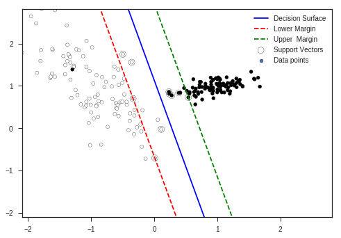
You can see in the plot that some data points have entered the forbidden area though according to our explanation this shouldn’t happen. But complex optimization and using many constraints enable this flexibility to \(SVM\)s so that they will be more robust to near margin noise.

Other notes on \(SVM\):

• If none of the training data fall within the margin of the classifier and a linear assumption ( as of now ) is true , then this classifier will be a very robust classifier. This is because the solution (\(\beta's\)) depend only on the support vectors not on other points. So it is immune to noise.

• On the other hand if a stochastic process is generating data points and if the points fall well within the margin of the classifier. It can affect the classifier very well since we gave no allowance to any datapoints in any class to be present within the margin.

• To accommodate the noisy data point ( possibly ) it will shrink the margin and thereby lose its robust nature.

• Classifiers that take not only support vectors, but those that take the entire dataset to find the distribution will be more accurate in this case.

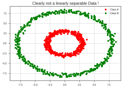
Kernel Transformations

What if the data is not linearly separable ?

Transform the data so that it becomes linearly separable !!!!

What do you mean by a transform ??

r1 = 3

r2 = 8
std = 0.25

t = np.linspace(0, 2*np.pi, 500)

x_1 = r1*np.cos(t) + std*np.random.randn(len(t))
y_1 = r1*np.sin(t) + std*np.random.randn(len(t))

x_2 = r2*np.cos(t) + std*np.random.randn(len(t))
y_2 = r2*np.sin(t) + std*np.random.randn(len(t))

plt.plot(x_1, y_1, 'ro', label = 'Class A')
plt.plot(x_2, y_2, 'go', label = 'Class B')
plt.legend(loc = 'best')
plt.grid(True)
plt.title("Clearly not a linearly separable Data !", fontsize = 16)
plt.show()

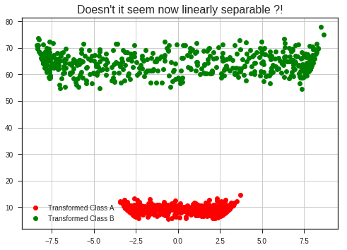
Now applying the following transformation,

\[\begin{equation} z = x^2 + y^2 = f(x,y) \end{equation}\]

We’ll be able to see something pretty amazing!

plt.plot(x_1, x_1**2 + y_1**2, 'ro', label = 'Transformed Class A')
plt.plot(x_2, x_2**2 + y_2**2, 'go', label = 'Transformed Class B')
plt.legend(loc = 'best')
plt.grid(True)
plt.title("Doesn't it seem linearly separable now?!", fontsize = 16)
plt.show()
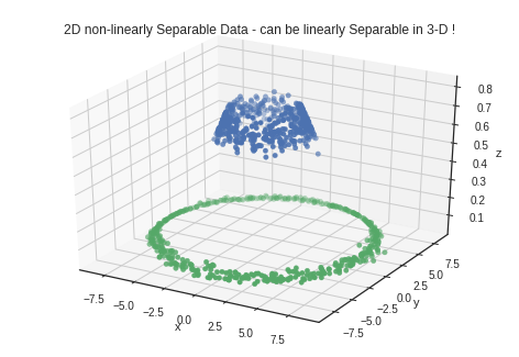
fig = plt.figure()
ax = fig.add_subplot(111, projection = '3d')
ax.scatter(x_1, y_1, x_1**2 + y_1**2, 'ro')
ax.set_xlabel('x')
ax.set_ylabel('y')
ax.set_zlabel('z')
ax.scatter(x_2, y_2, x_2**2 + y_2**2, 'go')
# ax.scatter(x_2, y_2, np.zeros_like(x_2))
plt.title("2D non-linearly Sepa.able Data - can be linearly Separable in 3-D !")
plt.show()

from mpl_toolkits.mplot3d import Axes3D
def gaussian(x,y, mu_x = 0,mu_y = 0, sigma_x = 5, sigma_y = 5, A = 1):
  return (A*(np.exp(-((x-mu_x)**2/(sigma_x**2)) + -((y-mu_y)**2/(sigma_y**2)))))
fig = plt.figure()
ax = fig.add_subplot(111, projection = '3d')
ax.scatter(x_1, y_1, gaussian(x_1, y_1), 'ro')
ax.set_xlabel('x')
ax.set_ylabel('y')
ax.set_zlabel('z')
ax.scatter(x_2, y_2, gaussian(x_2, y_2), 'go')
# ax.scatter(x_1, y_1, np.zeros_like(x_1))
plt.title("2D non-linearly Separable Data - can be linearly Separable in 3-D !")
plt.show()

These kind of transformations can be done on the data to make it linearly separable. Such transformations are called Kernel Transformations. Some popular examples are

• Polynomial Kernel: \((1 + \langle x,x^{'} \rangle )^d\)
• Radial Basis Function: \(e^{-\gamma \|x-x^{'}\|^{2}}\)
• Artificial Neural Network: \(tanh(k_1 \langle x, x^{'} \rangle + k_2)\)

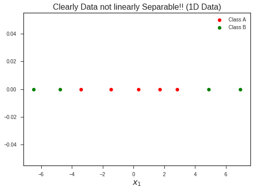
To understand how Kernel Transformations work, we will look into a simple example of Polynomial kernel.

x1 = np.linspace(-3, 3, 5) + 0.25*np.random.randn(len(np.linspace(-3, 3, 5)))
x2 = np.linspace(5, 7, 2)  + 0.25*np.random.randn(len(np.linspace(5, 7, 2)))
x3 = np.linspace(-5, -7, 2)  + 0.25*np.random.randn(len(np.linspace(-5, -7, 2)))
x2 = np.c_[x2, x3].flatten()
plt.plot(x1, np.zeros_like(x1), 'ro', label = 'Class A')
plt.plot(x2, np.zeros_like(x2), 'go', label = 'Class B')
plt.title("Clearly Data not linearly Separable!! (1D Data)", fontsize = 16)
plt.xlabel(r'$$x_1$$', fontsize = 16)
plt.legend(loc = 'best')
plt.show()

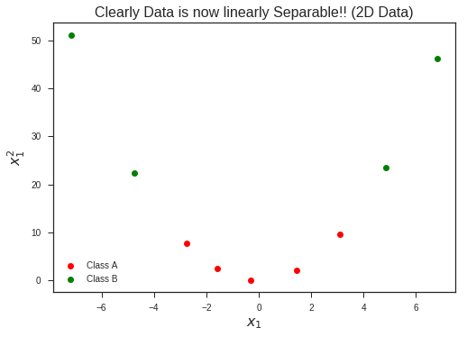
Increasing the dimentionality of the problem, now lifting this 1-D dataset to 2-D problem by introducing a new feature…

plt.plot(x1,x1**2, 'ro', label = 'Class A')
plt.plot(x2, x2**2, 'go', label = 'Class B')
plt.title("Clearly Data is now linearly Separable!! (2D Data)", fontsize = 16)
plt.xlabel(r'$$x_1$$', fontsize = 16)
plt.ylabel(r'$$x_1^2$$', fontsize = 16)
plt.legend(loc = 'best')
plt.show()