Summer School Deep Learning Session 3

An introduction to Convolutional Neural Networks

In this post we will be giving an introduction to Convolutional Neural Networks and will show you how to implement one.

The session notebook can be found here

Neurons as Feature Detectors

Recall how a neuron’s value is calculated. It consists of an aggregation and an activation step. It takes several real numbers as input and outputs a single real number. \begin{equation} Aggregation: Agg=b_1x_1 + b_2x_2 + \cdots + b_nx_n \end{equation} \begin{equation} Activation: y=\sigma(Agg) \end{equation} Note that the parameters of this neuron are \(b_i\) and are \(n\) in number. You may recall from JEE math that the aggregation step can be written as a dot product: \begin{equation} Agg=b\cdot x= |b||x|cos(\theta) \end{equation}

Where \(b\) and \(x\) are column vectors and \(\theta\) is the angle between them. For fixed magnitudes, the aggregate will be maximised when the angle between them is 0. In other words, the aggregattion step measures the similarity between \(x\) and \(b\) (specifically the cosine similarity). When the aggregation is large and positive, the neuron’s activation will approach 1 while if they are very dissimilar, the neuron should approach 0. Thus, a neuron can be interpreted as a feature detector. Presence of the feature in the input is indicated by the value of the neuron’s output.

There is a catch, however. In the preceding section, we assumed that the magnitudes of \(x\) and \(b\) were fixed. It is reasonable to ignore the magnitude of \(b\) since we are only interested in comparing the ‘strength’ of the feature’s presence across different values of \(x\). Ignoring the magnitude of \(x\) is dubious because we could drive the aggregate to a large value simply by letting all the elements of \(x\) be large values. This is why it is important to scale your data before passing it to any learning algorithm.

Images and Feed Forward Neural Networks

Suppose we want to use a neural network to classify images. An image consists of pixel values arranged in a matrix whose shape matches the resolution of the image. Since each pixel has a separate value for red, green and blue levels, you can imagine them as 3 matrices stacked up (3 channels). In order to use the image as input to the neural network from the last class, we need to transform this data into a 1-D vector. You should notice that the neural network we’ve been studying so far does not care about the ordering of the input vector, as long as all samples are ordered the same way. This order-independence allows us to squash our image in any way we want as long as we use the same method of squashing for each image in our dataset.

For simplicity, we will use grayscale images, which only require 1 matrix to store pixel values. Our squashing method is placing rows of the image next to each other.

The FMNIST dataset contains 60000 images in 10 classes:

T-shirt/top , Trouser , Pullover , Dress , Coat , Sandal , Shirt , Sneaker , Bag , Ankle boot

Thinking back to our feature detector discussion, consider a neuron in the first hidden layer. It has 784 inputs, each associated with a weight. The output of the neuron measures the similarity of the 784 inputs to the weights. If we plot these weights in a 28x28 image, we can see what feature the neuron is detecting. Here are the filters learned for 0 hidden layers. (green=positive, red=negative)

The case of zero hidden layers is equivalent to logistic regression. Let us plot the weights learned for a network with a single hidden layer.

We see that the first layer learns many duplicate features

Neurons in subsequent layers can be analysed similarly, however plotting them will not yield very interpretable information.

These neurons are actually looking for combinations of features from the first layer that result in more abstract representations of the input. For example, the first layer might detect similarity to circles and squares while the next layer could combine be active when both those neurons are active.

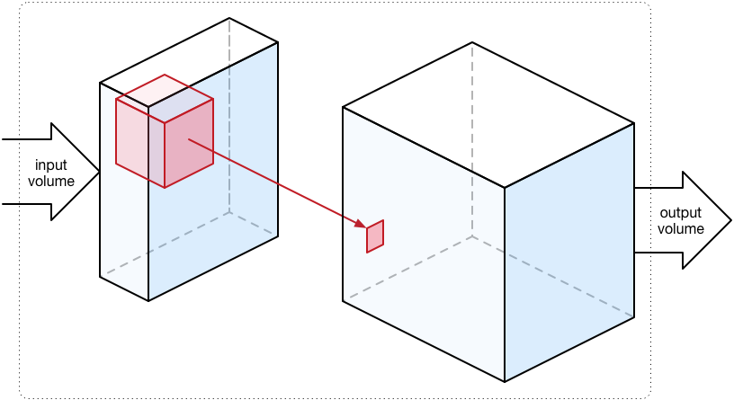
Convolution and Spatial Proximity In the previous section, we were measuring the similarity of the image to a learned weight matrix. But what would happen if the object we are trying to detect doesn’t overlap significantly with the learned weights? What if our object of interest is in the corner of the image? The detector neuron would not be activated and we would not detect the object.

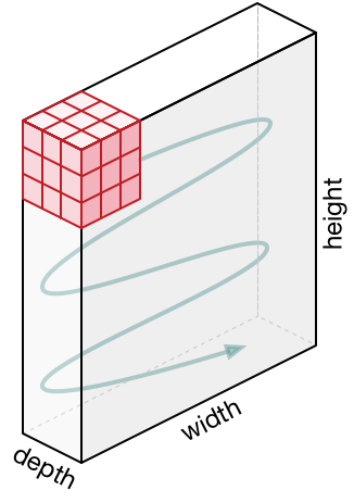
We could instead break the image into smaller pieces and look for parts of the object. This is what the convolution operator attempts to do. In the previous section, we looked to match the image with a 28x28 weight matrix. Why not look at every possible 5x5 square in the image and match it to a learned ‘filter’ of the same size?

The calculation we are performing is the same as before. we are simply doing it in patches of the image. The operation of performing this dot product over all patches of the image is known as convolution. Each dot product yields a real number, so the convolution operator outputs a matrix of these scalars.

Above is the output of the 8 Kirsch filters that find edges oriented along the compass directions.

One advantage convolution offers over a feed forward network is that it greatly reduces the parameters to be learned. We have gone from learning a 28x28 filter to learning a 5x5 filter for a single neuron. That amounts to a reduction by a factor of 30. The disadvantage is that this filter, being so small, cannot capture very complex information about the image. At best we can find edges in the first layer. As before, the network will detect more complex features in the deeper layers. It could use a vertical edge and a horizontal edge to determine whether there is a T shape in the image.

For images, CNNs usually perform better than feed forward nets even though CNNs have fewer parameters. Further, CNNs can be represented equivalently as feed forward nets. Why can’t a feed forward net learn this equivalent weight matrix that the CNN learns? The answer probably lies in spatial connectivity. The convolution operator inherently depends only on the neighbours of a pixel and we know naturally that a pixel must always be considered in the context of its neighbours in order to characterise it appropriately. CNNs are forced into doing this while a feedforward net would have to learn this on its own and with a massive parameter search space, this is highly unlikely to happen.

The Details of Convolution

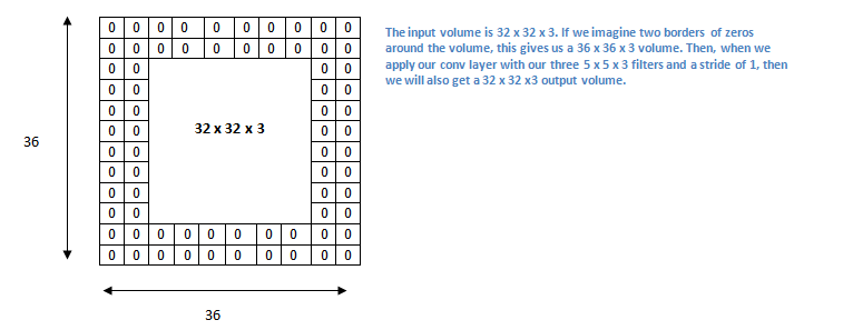
Padding

Notice in the gif above that the output matrix is smaller than the input matrix. This happens because the filter is not allowed to exceed the bounds of the image and can result in incomplete usage of features located near the edge of the image and is a waste of valuable data. There are a few ways to overcome this by using padding. Padding refers to adding dummy pixels around the image so as to ensure that the convolution does not change the size of the output matrix. A few forms of padding are ’constant’, ’nearest’, ’mirror’ and ‘wrap’.

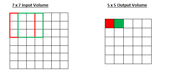
Stride

In our example, we’ve been shifting the filter 1 unit right before every dot product. If we instead move it by 2 units, the size of the output would reduce by a factor of 2. The amount by which the filter moves is known as the stride and can be adjusted to decrease the amount of computation required in subsequent layers.

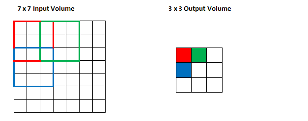
Now, let us increase the stride to 2.

Shift equivariance

Consider the case below where the same image is shifted and fed into some convolution operator. Notice that the output contains the same pattern of activations shifted by the same amount as the original image was shifted. This is known as translational equivariance. Convolutions are often misrepresented as being shift invariant but this is not the case since we can see that shifting the input does indeed change the output.

Handling Multiple Channels

Earlier, we assumed that the input to our convolution was a grayscale image which can be represented as a single matrix, rather than an rgb image which must be represented as a stack of matrices. How does convolution handle this? Instead of learning a filter matrix, we can learn 3 filter matrices (one for each channel) and stack them, creating a 3x3x3 filter. This is called a tensor.

The tensor moves across the image in the same way as before, performing a dot product and giving a matrix output after passing over the entire image. Convolution is therefore a tensor to matrix operation.

Handling Multiple Filters

Given an image, we would like to extract as much information about it as possible. We might want to find all the different oriented edges separately (similar to the kirsch operator). This would involve using many filters at once. Since each filter outputs a matrix, it is fairly straightforward to stack these matrices giving a tensor with \(f\) channels (where \(f\) is the number of filters). Let’s put all of this together and see what a convolution with multiple input and output channels looks like.

Building a CNN

Series Convolution

Now that we’ve seen how convolutions work, we can start to construct a neural network. The key idea here is to apply several convolutions in series so as to detect more and more nuanced features as we get deeper into the network. Why would this happen at all? We can show by a simple example that series convolutions can detect shapes in an image.

Let’s say we want to detect squares in our image. we could first use a kirsch filters to find the edges of the square first. The next set of convolutions can find whether these edges are perpendicular to each other and locate crossings. The next layer could convolve with a filter detecting 4 dots. This is a really simple example to show that features are heirarchical. We first detected edges, then combinations of edges and then shapes. Further layers can even detect textures.

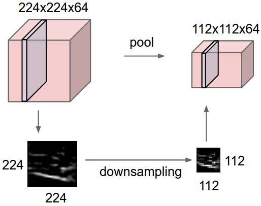
Pooling

A weakness of this method is that it isn’t scale invariant. This wouldn’t be able to detect squares of all sizes. 2 solutions to this are possible. The first solution would be to increase the stride of our filter so that spatially distant features in the image are brought closer together in the resulting feature map. As we go deeper into the network, feature maps would get smaller and smaller. The second way of going about this would be to perform a down sampling of the features maps at each stage. This is known as pooling. There are various methods of pooling like average and median, but the most common is called max pooling.

Max pooling involves moving a box over contiguous areas of the feature map and selecting the max value in boxes. The strides of the boxes are generally equal to the size of the boxes. 2x2 max-pooling is very common in deep learning. It is also non-parametric so it doesn’t need to learn any features to perform its operations, unlike filter convolutions. This is why most people prefer this method.

In addition to bringing us closer to scale invariance, max pooling is robust to small shifts in the image, therefore we have also taken a step in the direction of translation invariance.

Fully Connected Layers

Convolutions suffer from an inherent bias: they only take into account the neighbourhood of a pixel. if we were for example trying to detect a car in a high resolution image, the network would have to perform multiple down samplings until a single filter is able to cover 2 active wheel detector neurons. We could instead use fully connected layers to take note of these distributed features.

Putting it all together

CNNs over the years

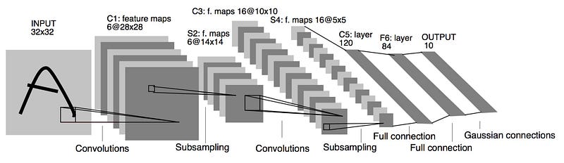
LENET5

It is the year 1994, and this is one of the very first convolutional neural networks, and what propelled the field of Deep Learning.

This pioneering work by Yann LeCun was named LeNet5 after many previous successful iterations since they year 1988.

IMAGENET

ImageNet Large Scale Visual Recognition Challenge (ILSVRC) evaluates algorithms for object detection and image classification at large scale. One high level motivation is to allow researchers to compare progress in detection across a wider variety of objects – taking advantage of the quite expensive labeling effort. Another motivation is to measure the progress of computer vision for large scale image indexing for retrieval and annotation.

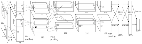
ALEXNET

In 2012, Alex Krizhevsky released AlexNet which was a deeper and much wider version of the LeNet and won by a large margin the difficult ImageNet competition.

Wide as in 20+% !

VGG

The VGG networks from Oxford were the first to use much smaller 3×3 filters in each convolutional layers and also combined them as a sequence of convolutions.

This seems to be contrary to the principles of LeNet, where large convolutions were used to capture similar features in an image.

Instead of the 9×9 or 11×11 filters of AlexNet, filters started to become smaller, too dangerously close to the infamous 1×1 convolutions that LeNet wanted to avoid, at least on the first layers of the network.

But the great advantage of VGG was the insight that multiple 3×3 convolution in sequence can emulate the effect of larger receptive fields, for examples 5×5 and 7×7. These ideas will be also used in more recent network architectures as Inception and ResNet.

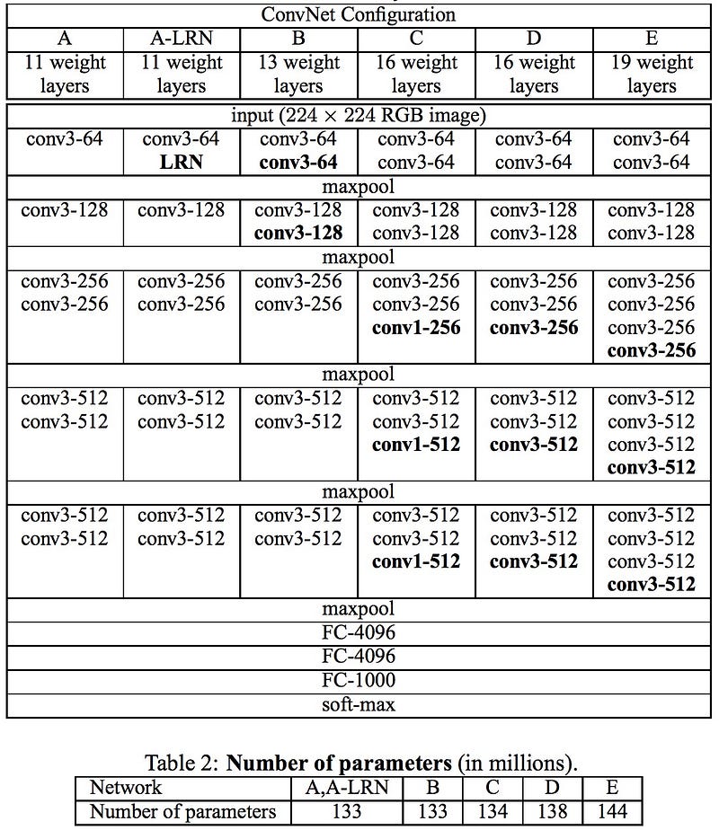
The VGG networks uses multiple 3×3 convolutional layers to represent complex features.

Notice blocks 3, 4, 5 of VGG-E: 256×256 and 512×512 3×3 filters are used multiple times in sequence to extract more complex features and the combination of such features.

This is effectively like having large 512×512 classifiers with 3 layers, which are convolutional! This obviously amounts to a massive number of parameters, and also learning power.

But training of these network was difficult, and had to be split into smaller networks with layers added one by one. All this because of the lack of strong ways to regularize the model, or to somehow restrict the massive search space promoted by the large amount of parameters.

VGG used large feature sizes in many layers and thus inference was quite costly at run-time. Reducing the number of features, as done in Inception bottlenecks, will save some of the computational cost.

GoogleNet and Inception

Let the Games begin XD

Christian Szegedy from Google begun a quest aimed at reducing the computational burden of deep neural networks, and devised the GoogLeNet the first Inception architecture.

By now, Fall 2014, deep learning models were becoming extermely useful in categorizing the content of images and video frames.

Most skeptics had given in that Deep Learning and neural nets came back to stay this time. Given the usefulness of these techniques, the internet giants like Google were very interested in efficient and large deployments of architectures on their server farms.

INCEPTION V3 (AND V2)

In February 2015 Batch-normalized Inception was introduced as Inception V2.

Batch-normalization computes the mean and standard-deviation of all feature maps at the output of a layer, and normalizes their responses with these values. This corresponds to “whitening” the data, and thus making all the neural maps have responses in the same range, and with zero mean. This helps training as the next layer does not have to learn offsets in the input data, and can focus on how to best combine features.

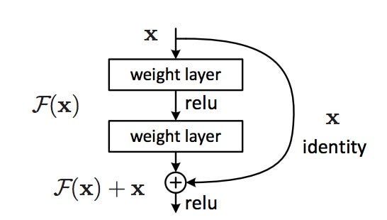
RESNET

The revolution then came in December 2015, at about the same time as Inception v3. ResNet have a simple ideas: feed the output of two successive convolutional layer AND also bypass the input to the next layers!

Inception v4 or Inception_Resnet_v2

1. List item
2. List item

There’s no method to this madness

And Christian and team are at it again with a new version of Inception.

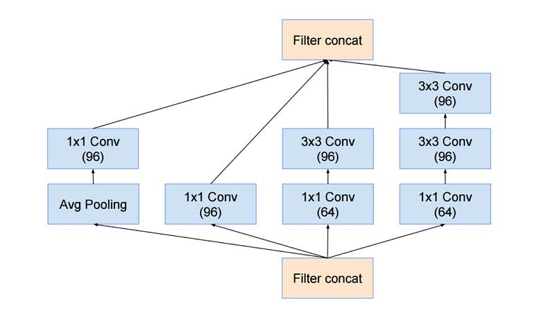
The Inception module after the stem is rather similar to Inception V3:

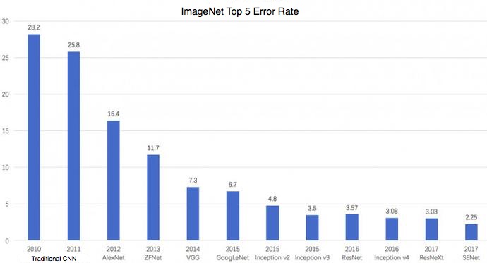
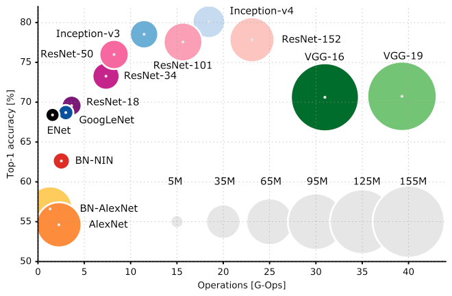
Convolutional Neural Networks’ Accuracy