Exploring Adversarial Reprogramming

Author: Rajat V D

This post was also posted on medium at Medium

Orginal post here

Google brain recently published a paper titled Adversarial Reprogramming of Neural Networks which caught my attention. It introduced a new kind of adversarial example for neural networks, those which could actually perform a useful task for the adversary as opposed to just fooling the attacked network. The attack ‘reprograms’ a network designed for a particular task to perform a completely different one. The paper showed that popular ImageNet architectures like Inception and ResNets can be successfully reprogrammed to perform quite well in different tasks like counting squares, MNIST and CIFAR-10.

I’m going to walk through the paper in this post, and also add some of my own small modifications to the work they presented in the paper. In particular, I experimented with a slightly different method of action of the adversarial program, different regularization techniques and also targeted different networks - ResNet 18 and AlexNet.

Paper summary

The paper demonstrated adversarial reprogramming of some famous ImageNet architectures like Inceptions v2, v3 and v4, along with some ResNets - 50, 101, and 152. They reprogrammed these networks to perform MNIST and CIFAR-10 classification, and also the task of counting squares in an image.

The gist of the reprogramming process is as follows:

• Take a pretrained model on ImageNet like Inception.
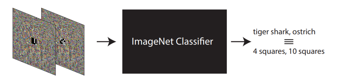
• Re-assign ImageNet labels to the labels of your target task. So for example, let ‘great white shark’ = 1 for MNIST, and so on. You can assign multiple ImageNet labels to the same adversarial label as well.
• Add an ‘adversarial program’ image to your MNIST image and pass that through the Inception model. Map the outputs of Inception using the remapping you chose above to get your MNIST predictions.
• Train only the adversarial program image on the remapped labels, while keeping the Inception weights frozen.
• Now you got yourself an MNIST classifier: Take an MNIST image, add on your trained adversarial program, run it through Inception, and remap its labels to get predictions for MNIST.

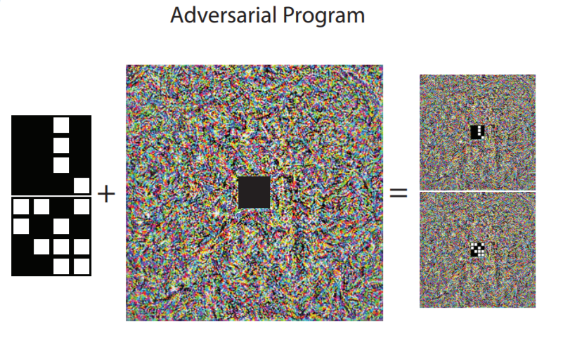
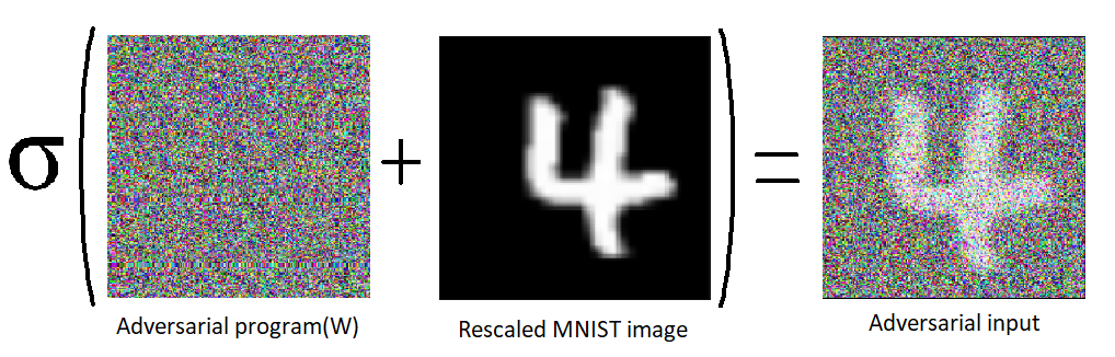
The exact method of ‘adding’ the adversarial program is as follows. Since ImageNet models require a 224 x 224 image, we use that as the size of our program weights. Let’s call the weights image \(W\). A nonlinear activation is applied to the weights after masking out the centre 28x28 section, which is then replaced by the MNIST image. This is the image which is passed in to our ImageNet model. Let’s define the mask with 0’s in the centre 28x28 as $M$. The adversarial input to the ImageNet model \(X_{adv}\) is:

\[X_{adv} = \tanh(W \odot M)+ pad(X)\]

where $\odot$ represents element wise multiplication, and $X$ is the input MNIST image. The illustrations in the paper shown below sum it up well:

Add a masked adversarial program to an input image from the counting squares task.

Pass through ImageNet model and remap outputs.

The outputs of the ImageNet model are trained using the cross-entropy loss as is normal for any classification problem. L2 regularization of the weight \(W\) was also done.

The results of the paper were quite interesting. Here are some important observations:

• They observed that using pre-trained ImageNet models allowed for a much higher accuracy than untrained or randomly initialized models(some models showed a disparity of ~80% test accuracy between trained and untrained).
• The adversarial programs for different models showed different qualitative features, meaning that they were architecture specific in some sense.
• Adversarially trained models showed basically no reduction in accuracy. This means that they are just as vulnerable to being reprogrammed as a normally trained model.

My Experiments

Regularization using blurring

One very important difference between these adversarial programs and traditional adversarial examples is that traditional examples were only deemed adversarial because the perturbation added to them was small in magnitude. However in this case, as the authors state, “the magnitude of this perturbation[adversarial program] need not be constrained”, as the adversarial perturbation is not applied on any previously true example. This fact is leveraged when training the program, as there are no limits on how large \(W\) can be. Another point to note is that the perturbation is a nonlinear function of the trained weights \(W\). This is in contrast to other adversarial examples like the Fast Gradient Sign Method which are linear perturbations.

One point which I’d like to bring up is that previous adversarial perturbations were better off if they contained high frequency components which made them “look like noise” (although they are anything but noise), as this resulted in perturbations which are imperceptible by the human eye. In other words, the perturbations did not change the true label of the image, but successfully fooled the targeted network. In the topic of adversarial programs however, there is no requirement for these perturbations to contain only high frequencies and be imperceptible, as the goal of the program is to repurpose the targeted network rather than to simply fool it. This means that we can enforce some smoothness in the trained program as a regularization technique as opposed to using L2 regularization.

I trained an adversarial program for ResNet-18 to classify MNIST digits using regularization techniques borrowed from this post. The basic idea is as follows:

• Blur the adversarial program image \(W\) after each gradient step using a gaussian blur, with a gradually decreasing sigma.
• Blur the gradients as well, again using a gaussian blur with gradually decreasing sigma.

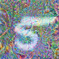
After training for around 20 epochs, this was the resulting adversarial program:

Animation and final result of training an adversarial program using masking for Resnet 18 on MNIST

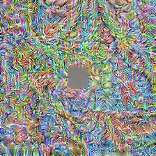
It managed a pretty high test accuracy of 96.81%, beating some of the networks described in the paper by a few points (this could be a property of Resnet 18 compared to the other networks they used). Note that I chose the output label mapping to some arbitrary ten labels of ImageNet(the paper used the first 10 labels), which had no relation with the MNIST digits themselves. We can see that there are interesting low frequency artifacts in the program image, which have been introduced due to the blurring regularization. We can also see the effect of reducing the blurring as the program develops finer details in the later part of the gif.

However, I do believe that this method of transforming the input using a mask is a bit lacking, so I tried my hand at a different input transformation.

Transforming by resizing

The authors of the paper mention that the input transformation and output remapping “could be any consistent transformation that converts between the input (output) formats for the two tasks and causes the model to perform the adversarial task”. In the case of the MNIST adversarial reprogramming, the input transformation was masking the weights and adding the MNIST input to the centre. The authors state that they used this masking “purely to improve visualization of the action of the adversarial program” as one can clearly see the MNIST digit in the adversarial image. The masking is not required for this process to work. This however seems a bit lacking in that the network is now forced to differentiate between the 10 MNIST classes using only the information in the center 28x28 pixels of the input, while the remaining part of the input, the adversarial program, remains constant for all the 10 classes. Another transformation which retains visualization ability is to simply scale the MNIST input (linearly interpolate) and add it to the adversarial program weights without any masking, before applying the non-linearity. In this case, the fraction of the adversarial input which distinguishes between classes is the same as that would be for any other MNIST classifier. An example is shown below:

Illustration of the input transformation described above.

Again, I trained an adversarial program using this new input transformation for Resnet 18. I used the same two regularization techniques of gradually decreased weight and gradient blurring as before, with the same parameters.

Animation and final result of training an adversarial program using scaling for Resnet 18 on MNIST.

An example of adversarial image obtained by adding a scaled version of the MNIST digit 5 to an adversarial program, and then applying a sigmoid activation. Resnet 18 classifies this image as an 'Egyptian Cat' with 0.99 confidence

The model obtained a test accuracy of 97.87%, around ~1% better than the masked transformation. It also obtained this accuracy after 15 epochs of training, showing faster convergence than the masked transformation. It also doesn’t sacrifice much in terms of visualization ability.

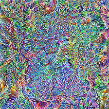
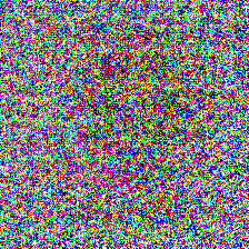
For comparisons, I also trained a program for a randomly initialized ResNet 18 network, using the gradient and weight blurring regularizations, and the scaling input transformation. As expected, the model performed much worse, with a test accuracy of only 44.15% after 20 epochs. The program also showed a lack of low frequency textures and features despite the use of blurring regularization:

Animation and final result of training an adversarial program for an untrained (randomly initialized) ResNet 18 network on MNIST even with blurring regularization

Multiple output label mappings

The above experiments have focused on changing the input transformation and regularization methods. I also experimented with using output label mappings which weren’t arbitrary. I experimented on this with CIFAR-10 because the task of reprogramming an ImageNet classifier to become a CIFAR-10 classifier are quite related. Both tasks have inputs which are photos of real objects, and their outputs are labels of these objects. It’s easy to find ImageNet labels which are closely related to CIFAR-10 labels. For example, the ImageNet label ‘airliner’ maps directly to the CIFAR-10 label ‘airplane’. To take a more structured approach, I ran the training images of CIFAR-10 (leaving aside a validation set) through ResNet 18 by rescaling to 224x224. This is equivalent to using an adversarial program which is initialized to 0. I then looked at the outputs of ResNet and compared them to the true labels of CIFAR-10. For this particular case, I performed multi-label mapping from ImageNet labels to CIFAR labels. In particular, I greedily mapped each ImageNet label to that CIFAR label which was classified the most by ResNet. In short:

• Run CIFAR train set through ResNet.
• Get a histogram of ImageNet labels for each CIFAR label.
• Map each ImageNet label to the CIFAR label with the highest value.
• For example, let’s look at the ImageNet label goldfish. After passing the CIFAR training set through the model, let’s say 10 trucks were classified as goldfish, 200 birds, 80 airplanes, etc. (these numbers are just examples). Suppose the 200 birds is the largest number of a single CIFAR class which was classified as goldfish. I then choose to map the goldfish output to the CIFAR label bird. This is the greedy part - I map the ImageNet label \(y\) to that CIFAR label which was classified as \(y\) the most often (in the training set). I repeat this process for all 1000 ImageNet labels.

To train the program with a multiple label mapping, I added the output probabilities of the multiple ImageNet labels corresponding to each CIFAR-10 label to get a set of 10 probabilities corresponding to each CIFAR label. I then used the negative log likelihood loss on these probabilities. Before going to the multi label mapping, I also trained an arbitrary 10 label mapping for ResNet 18 on CIFAR. It achieved a test accuracy of about 61.84% after 35 epochs. I then trained the same ResNet using the above greedy multi-label mapping with the same training parameters. It achieved a test accuracy of 67.63% after just 16 epochs.

Animation and final result of training an adversarial program using greedily chosen multiple output label mappings for Resnet 18 on CIFAR-10.

I repeated the above experiment on CIFAR-10 using AlexNet instead of Resnet 18. An arbitrary single output mapping yielded a test accuracy of 57.40% after 21 epochs, while using the greedy multi output mapping boosted that to 61.31% after 30 epochs.

Reprogrammed input of a CIFAR-10 truck which is classified by ResNet 18 as a 'trailer truck' with 0.42 confidence. Note that calling this input 'adversarial' is bit misleading, as this example can't really be considered one that 'fools' the target network.

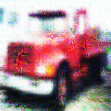
While we can keep chasing for percent points, note that CIFAR-10 is actually a bad example for demonstrating adversarial reprogramming, as the so called ‘adversarial’ inputs $X_{adv}$ aren’t really adversarial in the sense that the CIFAR labels are highly related to the ImageNet labels which have been greedily mapped. For example, the above figure shows an ‘adversarial’ input of a CIFAR-10 truck which is classified by ResNet 18 as a ‘trailer truck’. This isn’t really an adversarial input as the image could be considered as one of a trailer truck. However, the examples for CIFAR discussed in the paper in which the CIFAR image is put in the centre with a masked label can be considered adversarial, as a large part of these images cannot be interpreted meaningfully.

Testing Transferability

Another interesting thing to look at is whether these adversarial programs successfully transfer between different neural networks. In my experiments, it seemed that this was not the case. I tried using the MNIST adversarial program trained using ResNet 18 on AlexNet, and found that almost all the images were classified as ‘jigsaw puzzles’ irrespective of the digit they contained. Similar was the case for other ResNets like ResNet 34 and ResNet 50.

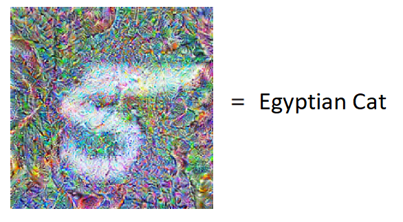
I also tried transferring the adversarial programs between the same networks but through a photograph on my phone. ResNet 18 classified a photo of the adversarial 5 as, again, a jigsaw puzzle as opposed to an Egyptian cat. This suggests that these adversarial examples are not very robust to noise, despite containing some low-frequency features. One possible reason for this could be that these examples occupy a niche in the adversarial example input space, as they were generated by training to fit a large dataset, however this remains a conjecture.

---

I wrote the code for all these experiments using PyTorch. Special thanks to my brother Anjan for the numerous discussions we had about these ideas and explorations.